15 降维

pacman::p_load(baguette, beans, bestNormalize, corrplot, discrim, embed, ggforce, klaR, learntidymodels, mixOmics, patchwork)

降维是指将高维数据映射到低维空间的过程。降维的目的是减少数据的维度，使得数据更易于理解和处理。

降维可用于特征工程或EDA中。
预测变量过多也会对模型产生不良的影响，例如共线性、变量间的高度相关性。
开始新的建模项目时，降维可能会提供一些关于建模难度的直观信息。

本章的目标在于：

如何使用recipe包穿件特征子集，并以此代表原始变量的主要特征。
如何单独使用recipe包，而不是将其整合进workflows中，这在测试不同预处理方法时很有用。但要注意，使用recipe的最佳方式还是将其整合进workflows中。

15.1 干豆品种数据集

干豆品种数据集中，一共记录了16个形态特征，包括面积、周长、偏心率等。部分特征具有高度的相关性，例如面积更大的物体通常会有更长的周长；此外，一个基本特征也会有很多量化的方法，例如衡量一个物体的大小，可以用面积、周长、高度等多种方法。

library(tidymodels)
tidymodels_prefer()

data(beans)

set.seed(1601)
bean_split <- initial_split(beans, prop = 3 / 4, strata = class)
bean_train <- training(bean_split)
bean_test <- testing(bean_split)

set.seed(1602)
bean_val <- initial_validation_split(bean_train, strata = class, prop = c(0.6, 0.2))

# 穿件颜色渐变的调色板函数
tmwr_cols <- colorRampPalette(c("#91CBD765", "#CA225E"))
bean_train %>%
  select(-class) %>%
  cor() %>%
  corrplot::corrplot(
    col = tmwr_cols(200), tl.col = "black", method = "ellipse"
  )

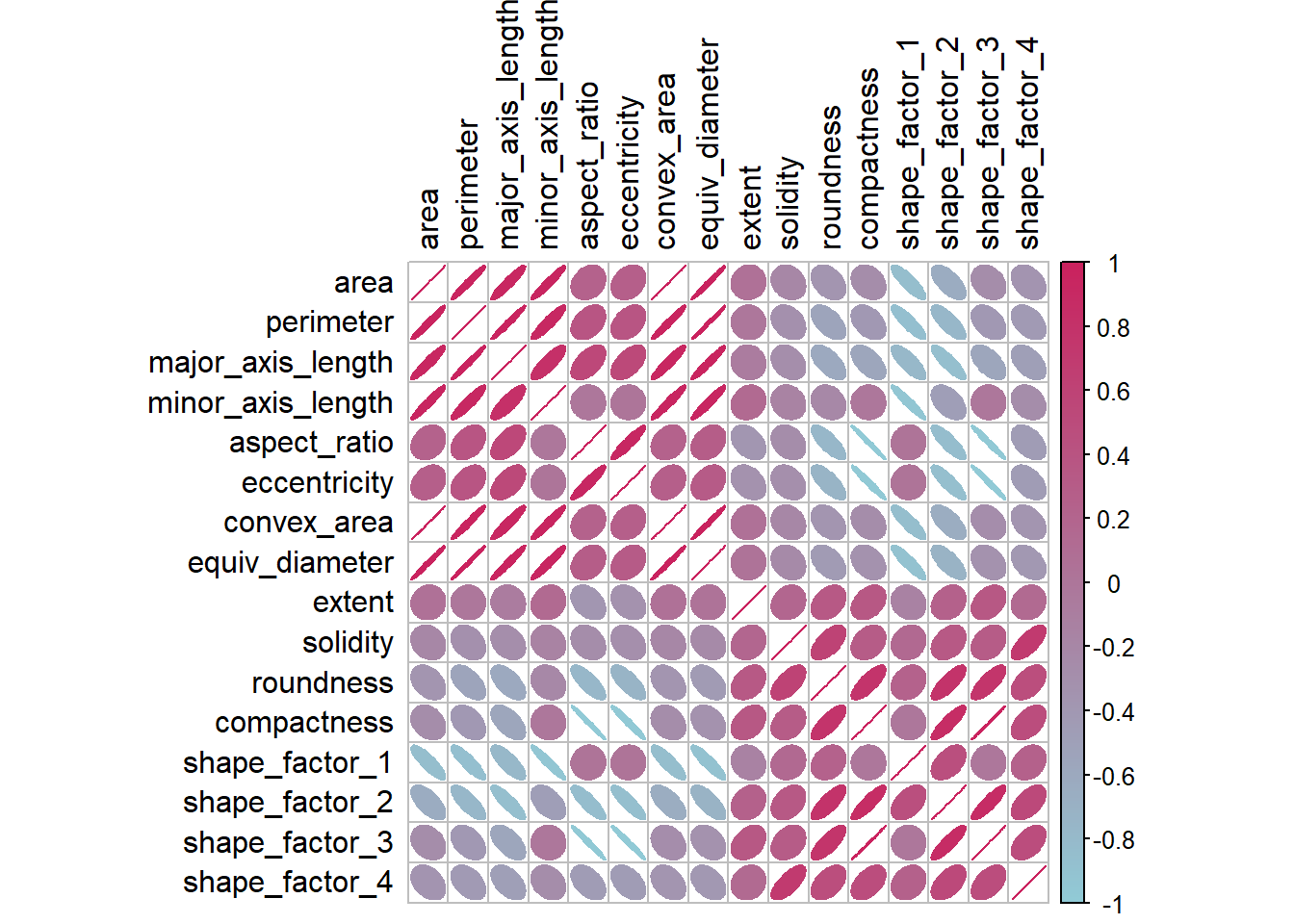
图 15.1 显示许多的预测变量之间是存在高度的相关性的。
除了探索相关性，还可以查看这种相关性在结果变量的不同类别中是否有显著不同。

15.2 recipe

15.2.1 建立基础recipe

bean_recipe <-
  # 使用bean_var中的训练集数据
  recipe(class ~ ., data = training(bean_val)) %>%
  step_zv(all_numeric_predictors()) %>% # 移除仅包含单个值的变量
  bestNormalize::step_orderNorm(all_numeric_predictors()) %>% # 强制预测变量为对称分布
  step_normalize(all_numeric_predictors())

15.2.2 单独使用recipe

回忆下，包含recipe的workflow可以使用fit()函数拟合模型(同时执行预处理步骤)，然后使用predict()函数对新数据执行同样的预处理步骤，并用拟合好的模型预测结果。如果我们还不希望拟合模型，只想看看当前的recipe应用在训练集/测试集上的结果时，就需要单独使用recipe。 - prep()函数类似fit()，对训练集执行预处理。 - 返回的是recipe对象，并展示了对哪些变量使用了哪种预处理步骤(Operations字段下)。 - prep()中的retain = TRUE参数可以将经过预处理的数据保留在返回的对象中，这样可以避免再次使用时进行的重复计算。但如果训练集很大，可以将本参数设定为FALSE。 - 在repice中增加新的预处理步骤后，重新调用prep()只会执行新增的预处理步骤。 - bake()函数对新数据/测试集执行预处理，返回的是tibble对象。类似predict()。 - 当prep()中的retain = TRUE时，bake()函数会直接返回recipe应用渔训练集后的数据集，这在训练集不是很大的时候很有用。 - bake()函数可以使用dplyr的变量选择器函数(selet(),starts_with()…来指定要返回的列，默认为everything()。

# prep()-准备recipe
bean_recipe_trained <- prep(bean_recipe, verbose = TRUE)

oper 1 step zv [training] 
oper 2 step orderNorm [training] 
oper 3 step normalize [training] 
The retained training set is ~ 0.77 Mb  in memory.

bean_recipe_trained

# bake()-使用/烘焙配方
bean_validation <- validation(bean_val)
bean_val_processed <- bean_recipe_trained %>%
  bake(bean_validation)

p1 <- bean_val_processed %>%
  ggplot(aes(x = area)) +
  geom_histogram(bins = 30, color = "white", fill = "blue", alpha = 0.3) +
  theme_minimal()

p2 <- bean_validation %>%
  ggplot(aes(x = area)) +
  geom_histogram(bins = 30, color = "white", fill = "blue", alpha = 0.3) +
  theme_minimal()

p2 + p1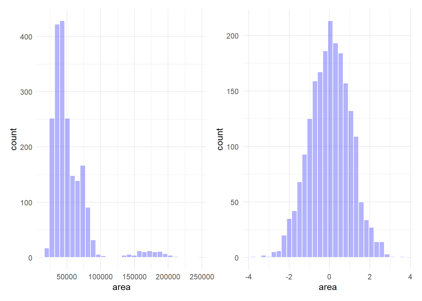

图 15.2 展示了bake()函数对新数据执行的预处理效果。可以看到，area变量的分布在预处理后基本对称。

15.3 特征提取技术

我们首先编写一个函数用于评估不同的降维方法并对评估结果进行可视化。

plot_validation_results <-
  function(recipe, dat = validation(bean_val)) {
    set.seed(1)
    plot_data <- recipe %>%
      prep() %>%
      # 处理数据-默认为验证集
      bake(new_data = dat, all_predictors(), all_outcomes()) %>%
      sample_n(250)

    # 把特征名变为符号以方便和!!一起使用
    nms <- names(plot_data)
    x_name <- sym(nms[1])
    y_name <- sym(nms[2])

    plot_data %>%
      ggplot(aes(
        x = !!x_name, y = !!y_name, color = class,
        fill = class, pch = class
      )) +
      geom_point(alpha = 0.9) +
      scale_shape_manual(values = 1:7) +
      coord_obs_pred() +
      theme_bw()
  }

15.3.1 主成分分析-PCA

主成分分析(PCA)是一种常用的降维技术，它通过线性变换将原始数据映射到一个新的坐标系中，新坐标系的坐标轴是原始数据中的主成分。PCA的目标是找到一个新的坐标系，使得数据在新坐标系中的方差最大。

recipe中使用step_pc()函数来执行PCA的预处理。

bean_recipe_pca <- bean_recipe_trained %>%
  step_pca(all_numeric_predictors(), num_comp = 4)
bean_recipe_pca %>%
  plot_validation_results() +
  ggtitle("PCA")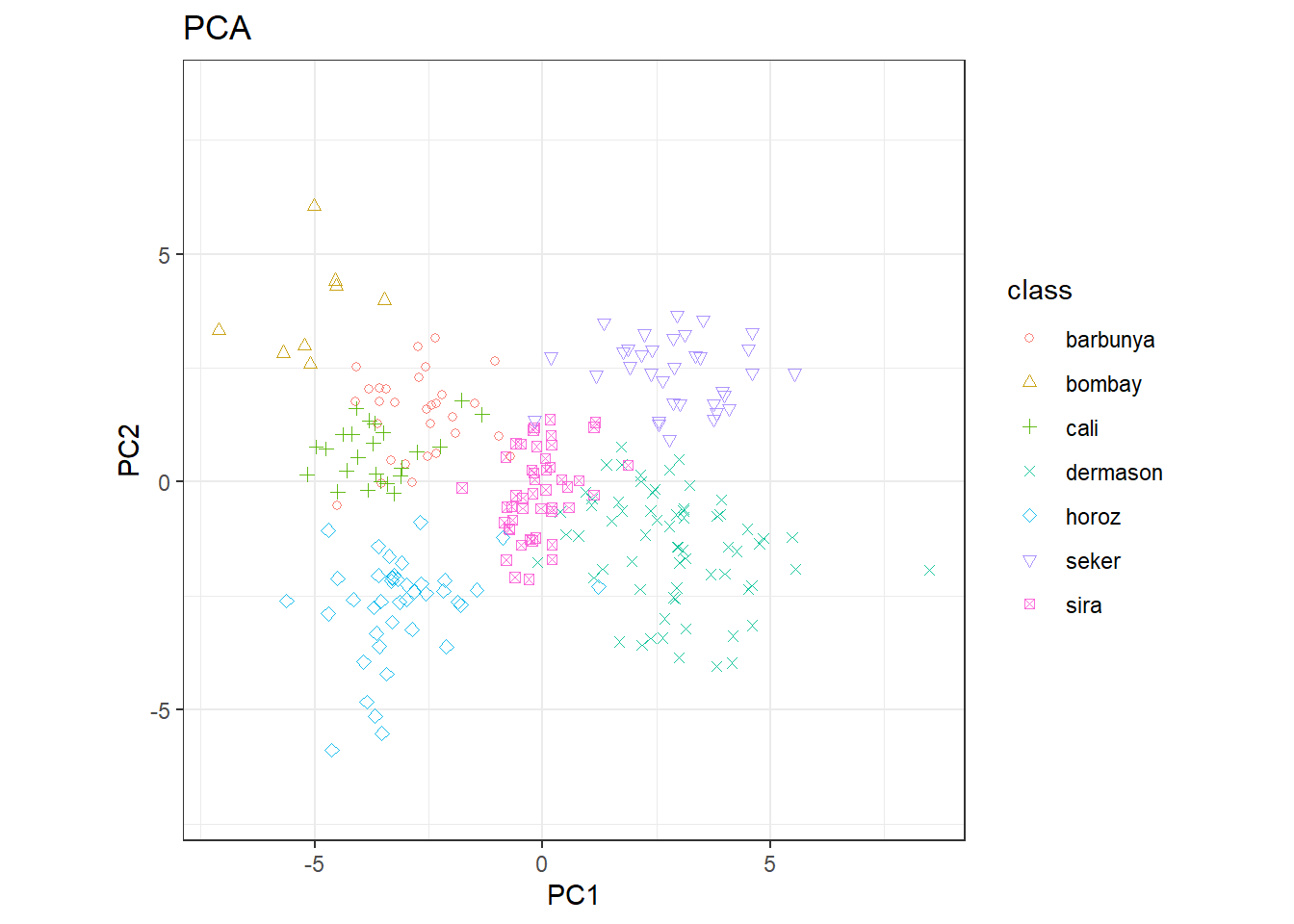

同时使用两个主成分能够比较清晰的区分出不同的类别。
可以合理猜测，对该数据集进行分类可能不会十分困难。

哪些变量对主成分的贡献最大呢？learntidymodels包的plot_top_loadings()函数可以可视化每个主成分的重要变量。

bean_recipe_trained %>%
  step_pca(all_numeric_predictors(), num_comp = 4) %>%
  prep() %>%
  learntidymodels::plot_top_loadings(component_number <= 4, n = 5) +
  scale_fill_brewer(palette = "Paired") +
  ggtitle("PCA predictors importance")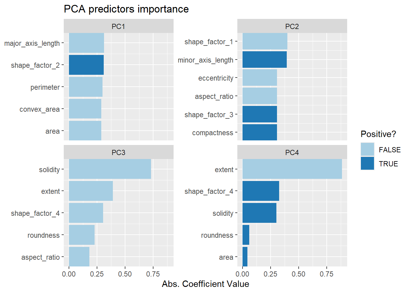

15.3.2 偏最小二乘法-PLS

PLS是PCA的有监督版本，通过向step_pls()函数中传递outcome参数实现有监督性。

bean_recipe_trained %>%
  step_pls(all_numeric_predictors(), outcome = "class", num_comp = 4) %>%
  plot_validation_results()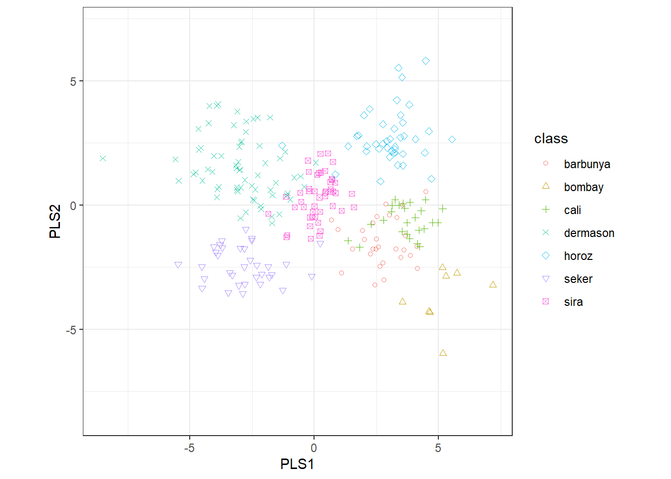

# pls各主成分变量重要程度
bean_recipe_trained %>%
  step_pls(all_numeric_predictors(), outcome = "class", num_comp = 4) %>%
  prep() %>%
  learntidymodels::plot_top_loadings(component_number <= 4, n = 5, type = "pls") +
  scale_fill_brewer(palette = "Paired") +
  ggtitle("PLS predictors importance")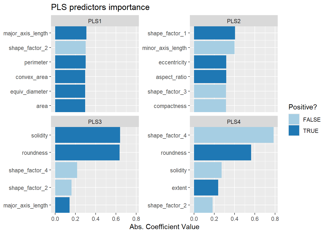

PLS和PCA前两个主成分的结果基本一致。

###　均匀流行近似和投影-UMAP

UMAP使用基于距离的最近邻方法寻找数据中数据点的相关性更大的局部区域。
UMAP对超参数非常敏感，需要一个优化过程。
embed::step_umap()函数实现，具有有监督和无监督两种算法，该函数有7个可供优化的超参数，具体可参见函数帮助文档的Tuneing Parameters部分。

p1 <- bean_recipe_trained %>%
  embed::step_umap(all_numeric_predictors(), num_comp = 4) %>%
  plot_validation_results() +
  ggtitle("UMAP")

p2 <- bean_recipe_trained %>%
  embed::step_umap(
    all_numeric_predictors(),
    outcome = "class", num_comp = 4
  ) %>%
  plot_validation_results() +
  ggtitle("UMAP(supervised)")

p1 + p2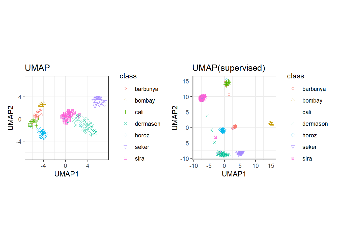

有监督的UMAP可以把结果非常清楚的区分。

15.4 建模

通过以上分析，PLS/PCA和UMAP方法都值得结合不同的模型开展进一步的研究。接下来，我们在多个模型中应用这两种降维方法并进行调优，使用的模型包括：单层神经网络、袋装数、柔性判别分析(FDA)、朴素贝叶斯和正则化判定分析(RDA)。

模型中的超参数和预处理中的超参数会一同调优。

library(baguette)
library(discrim)
# parsnip
mlp_spec <-
  mlp(hidden_units = tune(), penalty = tune(), epochs = tune()) %>%
  set_engine("nnet") %>%
  set_mode("classification")

bagging_spec <-
  bag_tree() %>%
  set_engine("rpart") %>%
  set_mode("classification")

fda_spec <-
  parsnip::discrim_flexible(
    prod_degree = tune()
  ) %>%
  set_engine("earth") %>%
  set_mode("classification")

rda_spec <-
  discrim_regularized(
    frac_common_cov = tune(),
    frac_identity = tune()
  ) %>%
  set_engine("klaR") %>%
  set_mode("classification")

bayes_spec <-
  naive_Bayes() %>%
  set_engine("klaR") %>%
  set_mode("classification")

# bacis recipe
bean_repice <-
  recipe(class ~ ., data = bean_train) %>%
  step_zv(all_numeric_predictors()) %>%
  bestNormalize::step_orderNorm(all_numeric_predictors()) %>%
  step_normalize(all_numeric_predictors())

# pls recipe
pls_recipe <-
  bean_recipe %>%
  step_pls(all_numeric_predictors(), outcome = "class", num_comp = tune())

# umap recipe
umap_recipe <-
  bean_recipe %>%
  embed::step_umap(
    all_numeric_predictors(),
    outcome = "class",
    num_comp = tune(),
    neighbors = tune(),
    min_dist = tune()
  )

# 建立workflowsets
bean_workflowsets <-
  workflow_set(
    preproc = list(
      basic = class ~ .,
      pls = pls_recipe, umap = umap_recipe
    ),
    models = list(
      bayes = bayes_spec, fda = fda_spec,
      rda = rda_spec, bag = bagging_spec,
      mlp = mlp_spec
    )
  )
bean_workflowsets

# A workflow set/tibble: 15 × 4
   wflow_id    info             option    result    
   <chr>       <list>           <list>    <list>    
 1 basic_bayes <tibble [1 × 4]> <opts[0]> <list [0]>
 2 basic_fda   <tibble [1 × 4]> <opts[0]> <list [0]>
 3 basic_rda   <tibble [1 × 4]> <opts[0]> <list [0]>
 4 basic_bag   <tibble [1 × 4]> <opts[0]> <list [0]>
 5 basic_mlp   <tibble [1 × 4]> <opts[0]> <list [0]>
 6 pls_bayes   <tibble [1 × 4]> <opts[0]> <list [0]>
 7 pls_fda     <tibble [1 × 4]> <opts[0]> <list [0]>
 8 pls_rda     <tibble [1 × 4]> <opts[0]> <list [0]>
 9 pls_bag     <tibble [1 × 4]> <opts[0]> <list [0]>
10 pls_mlp     <tibble [1 × 4]> <opts[0]> <list [0]>
11 umap_bayes  <tibble [1 × 4]> <opts[0]> <list [0]>
12 umap_fda    <tibble [1 × 4]> <opts[0]> <list [0]>
13 umap_rda    <tibble [1 × 4]> <opts[0]> <list [0]>
14 umap_bag    <tibble [1 × 4]> <opts[0]> <list [0]>
15 umap_mlp    <tibble [1 × 4]> <opts[0]> <list [0]>

ctrl <- control_grid(parallel_over = "everything")
# 设定并行计算选项
library(doParallel)
library(finetune)
registerDoParallel(core = round(parallel::detectCores() * 0.8))

bean_result <- bean_workflowsets %>%
  workflow_map(
    seed = 1603,
    resamples = validation_set(bean_val),
    grid = 10,
    metrics = metric_set(roc_auc),
    control = ctrl,
    verbose = TRUE
  )

rankings <- rank_results(bean_result, select_best = TRUE) %>%
  mutate(
    method = map_chr(wflow_id, \(x) str_split(x, "_", simplify = TRUE)[1])
  )
tidymodels_prefer()
filter(rankings, rank <= 5) %>%
  dplyr::select(rank, mean, model, method)

# A tibble: 5 × 4
   rank  mean model               method
  <int> <dbl> <chr>               <chr> 
1     1 0.995 discrim_regularized pls   
2     2 0.995 naive_Bayes         pls   
3     3 0.995 mlp                 pls   
4     4 0.994 mlp                 basic 
5     5 0.994 discrim_flexible    basic

rank_results(bean_result, select_best = TRUE) %>%
  mutate(
    method = map_chr(wflow_id, \(x) str_split(x, "_", simplify = TRUE)[1])
  ) %>%
  ggplot(aes(x = rank, y = mean, shape = method, color = model)) +
  geom_point(size = 5) +
  geom_text(
    aes(y = mean - 1 / 40, label = wflow_id),
    angle = 90, size = 5, hjust = 1
  ) +
  lims(y = c(0.4, 1.1))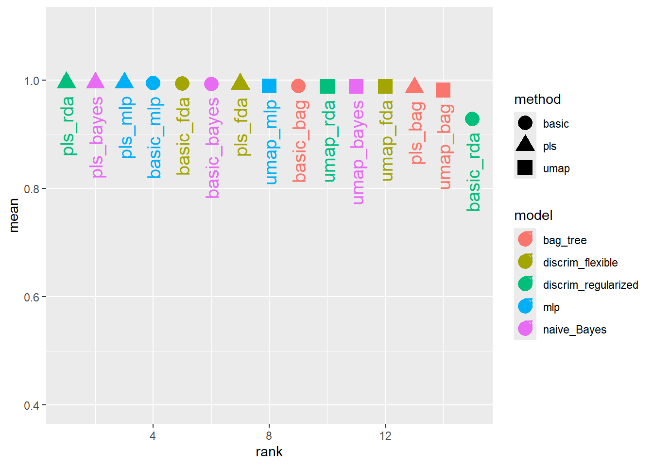

15.4.1 拟合最终模型

比较结果可以看出，大多数模型都提供了非常好的分类性能，且不同的与处理方案没有太大的区别。我们使用pls_rda模型作为最终模型进行演示。

# 提取最优模型的最优超参数
bean_final_result <- bean_result %>% 
  extract_workflow_set_result("pls_rda") %>% 
  select_best(metric = "roc_auc")

# 拟合最终模型
rda_res <- 
  bean_result %>% 
  extract_workflow("pls_rda") %>% 
  finalize_workflow(bean_final_result) %>%  # 将最优超参数应用至工作流
  last_fit(split = bean_split, metrics = metric_set(roc_auc))

predict(rda_res %>% 
  extract_workflow(),
  new_data = bean_test)

# A tibble: 3,405 × 1
   .pred_class
   <fct>      
 1 seker      
 2 seker      
 3 seker      
 4 seker      
 5 dermason   
 6 dermason   
 7 seker      
 8 seker      
 9 seker      
10 seker      
# ℹ 3,395 more rows

# 查看模型表现
collect_metrics(rda_res)

# A tibble: 1 × 4
  .metric .estimator .estimate .config        
  <chr>   <chr>          <dbl> <chr>          
1 roc_auc hand_till      0.995 pre0_mod0_post0