library(tidymodels)
library(tidyverse)
tidymodels_prefer()

mlp_spec <-
  mlp(hidden_units = tune(), epochs = tune(), penalty = tune()) %>%
  set_engine("nnet", trace = 0) %>%  # trace=0表示可以减少训练过程中的日志输出。
  set_mode("classification")

# 提取超参数
mlp_params <- mlp_spec %>%
  extract_parameter_set_dials()
mlp_params12 超参数调优的网格搜索法
在确定模型性能指标和重抽样方法后,下一个问题就是如何调优超参数。
超参数调优主要有两种方法:
- 网格搜索:本章学习网格搜索。
- 迭代搜索:在 Chapter 13 中介绍。
设定超参数网格的方法很灵活,在实际使用中可以根据实际情况选择自己喜欢的一种即可。
12.1 规则网格和不规则网格
在讨论更多细节之前,需要先建立一个需要超参数调优的多层感知机模型,改模型需要调整的超参数包括:
- 隐藏层数量:tidymodels中为
hidden_units。 - 模型拟合的epoch数量/迭代次数:tidymodels中为
epochs。 - 权重衰减惩罚值: tidymodels中为
penalty。
以上结果表明:
- 模型有3个超参数:
hidden_units,epochs,penalty。 - 每个超参数对象都是完整的,可以使用
extract_parameter_dials()函数提取单独的超参数及其默认取值范围。
12.1.1 规则网格
- 规则网格包含了每个超参数值的所有可能组合。
- 规则网格需要提前为每个超参数指定一组不同的值。
- 规则网格的优点是简单易懂,缺点是可能生成过多的组合,导致搜索时间过长。
-
dials::grid_**()系列函数可以生成超参数网格。其中grid_regular()函数可以生成规则网格。 参数levels用于指定每个超参数的取值数量,它可以接受一个整数或者一个命名向量。
# 每个超参数有两个取值的网格
grid_regular(mlp_params, levels = 2)
# A tibble: 8 × 3
hidden_units penalty epochs
<int> <dbl> <int>
1 1 0.0000000001 10
2 10 0.0000000001 10
3 1 1 10
4 10 1 10
5 1 0.0000000001 1000
6 10 0.0000000001 1000
7 1 1 1000
8 10 1 1000# 分别指定超参数的数量
grid_regular(
mlp_params,
levels = c(hidden_units = 3, penalty = 2, epochs = 2))# A tibble: 12 × 3
hidden_units penalty epochs
<int> <dbl> <int>
1 1 0.0000000001 10
2 5 0.0000000001 10
3 10 0.0000000001 10
4 1 1 10
5 5 1 10
6 10 1 10
7 1 0.0000000001 1000
8 5 0.0000000001 1000
9 10 0.0000000001 1000
10 1 1 1000
11 5 1 1000
12 10 1 100012.1.2 不规则网格
-
dials::grid_random()函数可以在超参数取值范围内生成独立且均匀的随机超参数值。随机网格的问题在于,中小规模的网格中,随机超参数的组合可能会有重叠。此外,如果需要随机网格覆盖整个超参数空间,则需要足够多的超参数值。 - 空间填充设计(space-filling designs)是一种更好的创建不规则网络的方法,
dials包提供了实现拉丁超立方和最大熵设计的函数。-
dials::grid_latin_hypercube()函数可以生成拉丁超立方网格。 -
dials::grid_max_entropy()函数可以生成最大熵网格。 - 在
tidymodels的1.3.0版本中,以上两个函数已经被grid_space_filling()函数取代,该函数的type参数可以指定网格类型。
-
library(ggforce)
set.seed(1303)
mlp_params %>%
  grid_space_filling(
    size = 10,
    original = FALSE,  # 是否使用转换后的超参数取值
    type = "latin_hypercube"
  ) %>%
  ggplot(aes(x = .panel_x, y = .panel_y)) +
  geom_point() +
  geom_blank() +
  facet_matrix(vars(hidden_units, penalty, epochs), layer.diag = 2)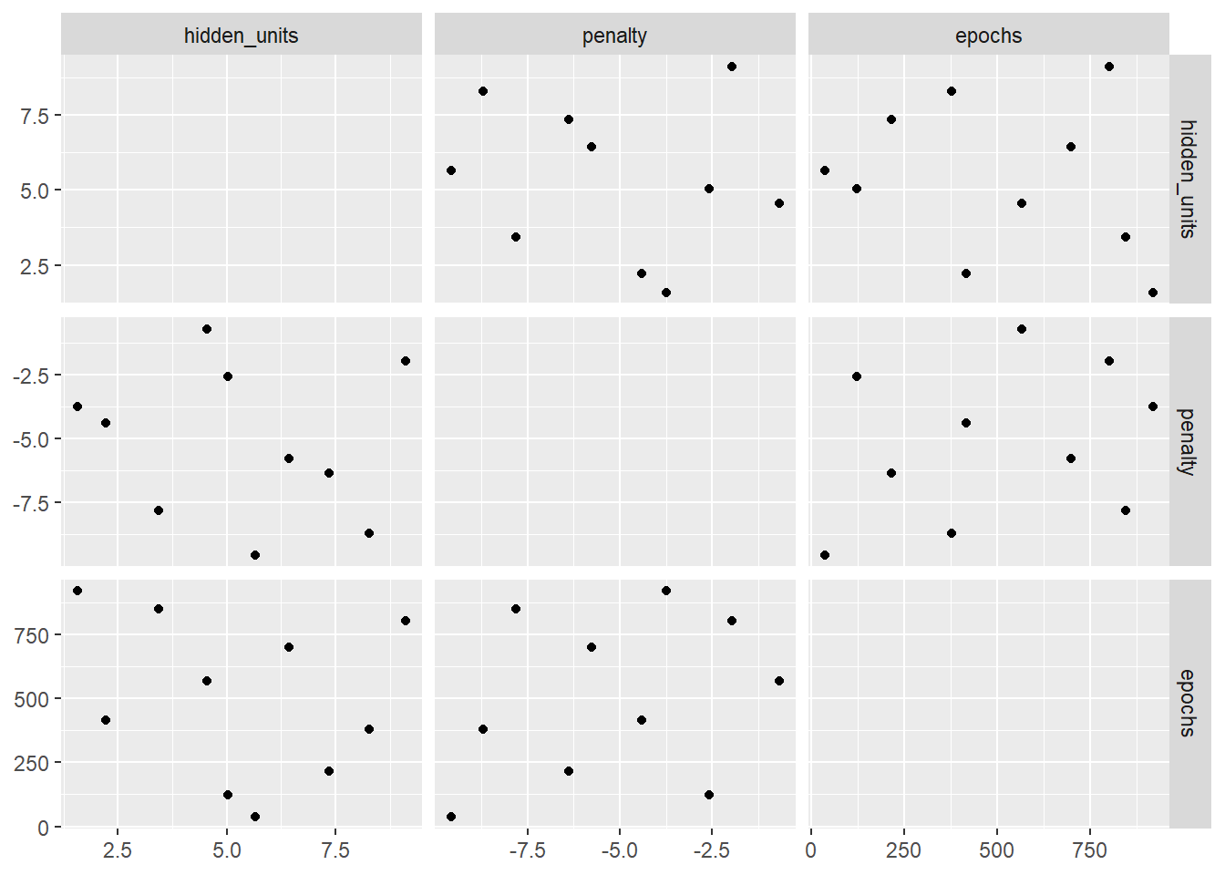
上图中网格每个点代表一个超参数组合。使用拉丁超立方网格生成的超参数组合点与点之间的距离更远,重合也更少,可以更好的探索超参数空间,可以极大的增加找到最优超参数组合的机会。
12.2 评估网格
- 使用重抽样评估不同的超参数组合后,就可以根据模型性能选择最合适的超参数组合了。
- 使用
cells数据集为例,该数据包含2019个人类乳腺癌细胞的56个图像测量值,数据集已知的信息如下:- 预测变量代表细胞不同部分的形状和强度特征(如细胞核、细胞边界等)。
- 预测变量之间存在强相关性。
- 本数据是实验室测试的一部分,因此构建模型的重点是模型的预测能力。
data(cells)
cells <- cells %>%
  select(-case)

# 创建重采样-使用10折交叉验证
set.seed(1304)
cell_folds <- vfold_cv(cells, v = 10)

# 使用PCA降维去除预测变量间的相关性
mlp_rec <-
  recipe(class ~ ., data = cells) %>%
  step_YeoJohnson(all_numeric_predictors()) %>%
  step_normalize(all_numeric_predictors()) %>%
  step_pca(all_numeric_predictors(), num_comp = tune()) %>%
  step_normalize(all_numeric_predictors())

# 建立workflow
mlp_wflow <-
  workflow() %>%
  add_recipe(mlp_rec) %>%
  add_model(mlp_spec)

# 创建超参数对象
mlp_params <- mlp_wflow %>%
  extract_parameter_set_dials() %>%
  update(
    epochs = epochs(c(50, 200)),
    num_comp = num_comp(c(0, 40))
  )

# 评估网格
set.seed(1305)
roc_res <- metric_set(roc_auc)
## 使用空间填充设计生成网格并评估
mlp_std_tune <-
  mlp_wflow %>%
  tune_grid(
    cell_folds,
    grid = 20,
    # 传递mlp_params以使用自定义的超参数范围
    param_info = mlp_params,
    metrics = roc_res # 指定评估指标,为一个`yardstick::metric_set()`对象
  )
mlp_std_tune
# Tuning results
# 10-fold cross-validation
# A tibble: 10 × 4
splits id .metrics .notes
<list> <chr> <list> <list>
1 <split [1817/202]> Fold01 <tibble [20 × 8]> <tibble [0 × 4]>
2 <split [1817/202]> Fold02 <tibble [20 × 8]> <tibble [0 × 4]>
3 <split [1817/202]> Fold03 <tibble [20 × 8]> <tibble [0 × 4]>
4 <split [1817/202]> Fold04 <tibble [20 × 8]> <tibble [0 × 4]>
5 <split [1817/202]> Fold05 <tibble [20 × 8]> <tibble [0 × 4]>
6 <split [1817/202]> Fold06 <tibble [20 × 8]> <tibble [0 × 4]>
7 <split [1817/202]> Fold07 <tibble [20 × 8]> <tibble [0 × 4]>
8 <split [1817/202]> Fold08 <tibble [20 × 8]> <tibble [0 × 4]>
9 <split [1817/202]> Fold09 <tibble [20 × 8]> <tibble [0 × 4]>
10 <split [1818/201]> Fold10 <tibble [20 × 8]> <tibble [0 × 4]>## 可视化评估结果-不规则网格
autoplot(mlp_std_tune) +
scale_color_viridis_d(direction = -1) +
theme(legend.position = "top")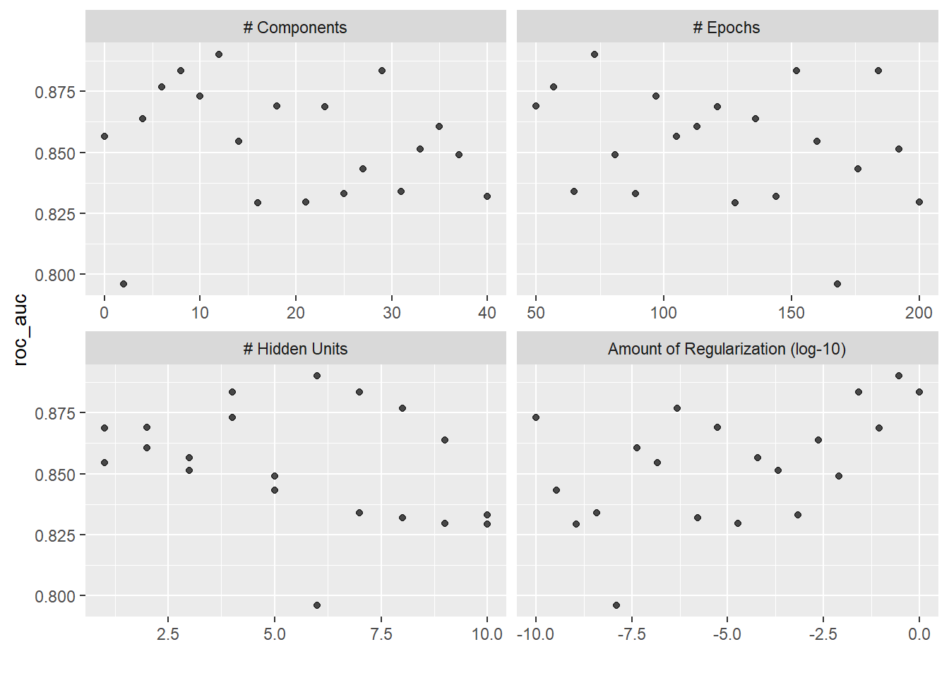
## 使用规则网格评估
mlp_reg_tune <-
  mlp_wflow %>%
  tune_grid(
    cell_folds,
    grid = grid_regular(mlp_params, levels = 3),
    metrics = roc_res
  )
mlp_reg_tune
# Tuning results
# 10-fold cross-validation
# A tibble: 10 × 4
splits id .metrics .notes
<list> <chr> <list> <list>
1 <split [1817/202]> Fold01 <tibble [81 × 8]> <tibble [0 × 4]>
2 <split [1817/202]> Fold02 <tibble [81 × 8]> <tibble [0 × 4]>
3 <split [1817/202]> Fold03 <tibble [81 × 8]> <tibble [0 × 4]>
4 <split [1817/202]> Fold04 <tibble [81 × 8]> <tibble [0 × 4]>
5 <split [1817/202]> Fold05 <tibble [81 × 8]> <tibble [0 × 4]>
6 <split [1817/202]> Fold06 <tibble [81 × 8]> <tibble [0 × 4]>
7 <split [1817/202]> Fold07 <tibble [81 × 8]> <tibble [0 × 4]>
8 <split [1817/202]> Fold08 <tibble [81 × 8]> <tibble [0 × 4]>
9 <split [1817/202]> Fold09 <tibble [81 × 8]> <tibble [0 × 4]>
10 <split [1818/201]> Fold10 <tibble [81 × 8]> <tibble [0 × 4]>## 可视化评估结果-规则网格
autoplot(mlp_reg_tune) +
scale_color_viridis_d(direction = -1) +
theme(legend.position = "top")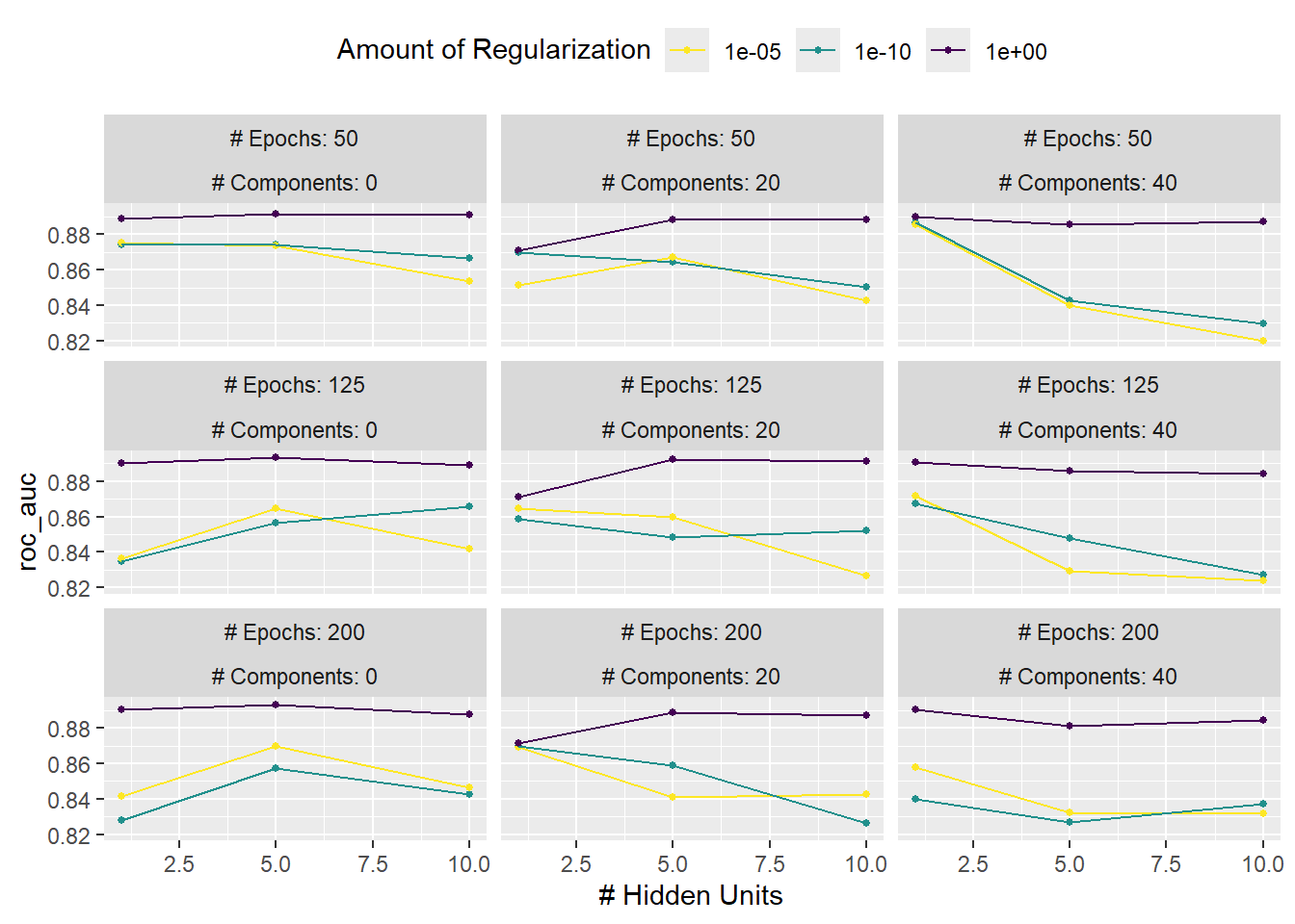
# A tibble: 5 × 9
  hidden_units      penalty epochs num_comp .metric  mean     n std_err .config
         <int>        <dbl>  <int>    <int> <chr>   <dbl> <int>   <dbl> <chr>
1            6 0.298            73       12 roc_auc 0.890    10 0.00991 pre07_m…
2            4 0.0264          184        8 roc_auc 0.883    10 0.00827 pre05_m…
3            7 1               152       29 roc_auc 0.883    10 0.0104  pre15_m…
4            8 0.000000483      57        6 roc_auc 0.877    10 0.00770 pre04_m…
5            4 0.0000000001     97       10 roc_auc 0.873    10 0.00738 pre06_m…
# A tibble: 5 × 9
hidden_units penalty epochs num_comp .metric mean n std_err .config
<int> <dbl> <int> <int> <chr> <dbl> <int> <dbl> <chr>
1 5 1 125 0 roc_auc 0.894 10 0.00851 pre1_mod17_p…
2 5 1 200 0 roc_auc 0.893 10 0.00808 pre1_mod18_p…
3 5 1 125 20 roc_auc 0.892 10 0.0104 pre2_mod17_p…
4 5 1 50 0 roc_auc 0.891 10 0.00868 pre1_mod16_p…
5 10 1 125 20 roc_auc 0.891 10 0.00867 pre2_mod26_p…以上代码的步骤包括:
-
step_YeoJohnson(),对所有数值型变量进行Yeo-Johnson变换,是所有预测变量的分布更加对称。 -
step_normalize(),对所有数值型变量进行标准化。 -
step_pca(),对所有数值型变量进行主成分分析,降维。其中num_comp参数用于指定降维后的主成分数量,是一个超参数。 -
step_normalize(),对降维后的数据再次进行标准化,是为了防止主成分分析引入的误差影响模型性能。 - 最后将
recipe和model整合至workflow中。 - 创建超参数对象并修改其中部分超参数的初始范围,
epochs和num_comp参数的取值范围分别设定为50200和040。 - 使用
autoplot()函数可视化不同超参数组合和性能指标之间的关系:- 本例中的评估指标采用的是
ROC-AUC曲线(纵坐标)。 - 规则网络下:不同颜色代表
epochs和num_comp相同情况下,惩罚值对评价指标的影响。可以看出惩罚值的大小对评价指标的影响最大;横坐标hidden_units``hidden_units对评价指标的影响随惩罚值增加而逐渐降低(横坐标曲线逐渐降低)。 - 通过
show_best()函数可以查看最优超参数组合。
- 本例中的评估指标采用的是
- 最好使用多个指标来评估超参数组合。此外,通常会选择一个次最优的超参数组合使模型的复杂度降低。
-
tune_grid()函数和fit_resamples()函数一样,默认不会保存训练过程中产生的模型。如果需要保存模型,可以设置control = control_grid(save_pred = TRUE)。这些结果可以使用collect_predictions()函数提取。
12.3 确定最终模型
有两种方式可以确定最终模型:
- 根据
tune_grid()函数的输出结果,手动选择适合的超参数值。 - 使用
select_****()系列函数选择最优的超参数组合。例如select_best()函数可以选择评价指标最好的超参数组合。 - 使用
finalize_workflow()将选择好的超参数组合应用到模型中,重新训练模型。如果没有定义工作流,那么可以使用finalize_recipe()或finalize_model()函数将选择好的预处理步骤或模型应用到数据中确定最终的模型。
manual_params <-
  tibble(
    hidden_units = 1,
    epochs = 125,
    penalty = 1,
    num_comp = 10
  )

# 应用至工作流
final_mlp_wflow <-
  mlp_wflow %>%
  finalize_workflow(manual_params)
final_mlp_wflow
══ Workflow ════════════════════════════════════════════════════════════════════
Preprocessor: Recipe
Model: mlp()
── Preprocessor ────────────────────────────────────────────────────────────────
4 Recipe Steps
• step_YeoJohnson()
• step_normalize()
• step_pca()
• step_normalize()
── Model ───────────────────────────────────────────────────────────────────────
Single Layer Neural Network Model Specification (classification)
Main Arguments:
hidden_units = 1
penalty = 1
epochs = 125
Engine-Specific Arguments:
trace = 0
Computational engine: nnet # 重新训练模型
final_mlp_fit <- final_mlp_wflow %>%
fit(cells)
final_mlp_fit══ Workflow [trained] ══════════════════════════════════════════════════════════
Preprocessor: Recipe
Model: mlp()
── Preprocessor ────────────────────────────────────────────────────────────────
4 Recipe Steps
• step_YeoJohnson()
• step_normalize()
• step_pca()
• step_normalize()
── Model ───────────────────────────────────────────────────────────────────────
a 10-1-1 network with 13 weights
inputs: PC01 PC02 PC03 PC04 PC05 PC06 PC07 PC08 PC09 PC10
output(s): ..y
options were - entropy fitting decay=112.4 创建调优设定的工具
-
usemodels包可以根据数据和模型公式,自动给出调优的R代码。它还会根据模型和数据类型自动给出合适的recipe,以满足模型的基本要求。 - 我们应自己设定重抽样方法和网格类型。
library(usemodels)

usemodels::use_xgboost(
  Sale_Price ~ Neighborhood + Gr_Liv_Area +Year_Built + Bldg_Type +
    Latitude + Longitude,
  data = ames_train,
  verbose = TRUE  # 添加注释以解释代码含义
)
xgboost_recipe <-
recipe(formula = Sale_Price ~ Neighborhood + Gr_Liv_Area + Year_Built + Bldg_Type +
Latitude + Longitude, data = ames_train) %>%
step_zv(all_predictors())
xgboost_spec <-
boost_tree(trees = tune(), min_n = tune(), tree_depth = tune(), learn_rate = tune(),
loss_reduction = tune(), sample_size = tune()) %>%
set_mode("classification") %>%
set_engine("xgboost")
xgboost_workflow <-
workflow() %>%
add_recipe(xgboost_recipe) %>%
add_model(xgboost_spec)
set.seed(66288)
xgboost_tune <-
tune_grid(xgboost_workflow, resamples = stop("add your rsample object"), grid = stop("add number of candidate points"))12.4.1 提升网格搜索效率
- 有很多可以提升效率的方法,我们着重介绍竞争法。通过分段式重采样来实现计算效率的提升,即先在一部分重抽样中评估模型,剔除表现较差的模型后,再进行后续的重抽样计算。
-
finetune::tune_race_anova()函数可以实现竞争法,并通过方差分析检验模型配置间的统计学显著性。基础的用法与tune_grid()相同。
library(finetune)

set.seed(1308)
mlp_std_race <-
  mlp_wflow %>%
  tune_race_anova(
    cell_folds,
    grid = mlp_params %>% grid_regular(levels = 3),
    metrics = roc_res,
    control = control_race(verbose_elim = TRUE)  # 显示剔除模型的过程
  )