2  假设检验

Chapter 1 中介绍了如何使用infer包进行抽样和置信区间的估计。本节我们继续使用infer包，介绍假设检验的基本流程和方法。

Appendix B 中有更多的实例说明假设检验。

pacman::p_load(
  tidyverse,
  moderndive,
  infer,
  nycflights23,
  ggplot2movies
)

表 2.1: 三种常用的差异性检验方法

X变量类型	X组别数量	Y变量类型	分析方法	R语法1
定类	2组或者多组	定量	方差（F检验）	aov()
定类	仅仅2组	定量	t检验	t.test()
定类	2组或者多组	定类	卡方	chisq.test()

值得注意的是，对于假设检验来说，重点关注置信区间比传统的理论方法更适合长期学习，也更符合新的理念。

2.1 将置信区间和假设检验联系起来

假设检验的基本步骤：

1. 确定零假设和备择假设。
2. 选择检验统计量。

• Z检验：大样本（n ≥ 30）或总体方差已知时，检验均值。
• t检验：小样本、总体方差未知时，检验均值。
• 卡方检验：检验方差或分类变量的独立性。
• F检验：比较两组方差是否相等（如ANOVA）。

3. 确定显著性水平 \(\alpha\)。
4. 计算检验统计量。
5. 根据统计量和显著性水平，判定零假设是否成立。

• 进行双侧检验时，p值为两个尾部的面积。
• 进行左侧检验时，p值为检验统计量左侧分布下的面积。
• 进行右侧检验时，p值为检验统计量右侧分布下的面积。

2.1.1 零假设和相关概念

• 零假设，顾名思义应为一个发生概率很小的极端事件，是我们希望证实事件的对立事件。例如希望证实一种药物对某种症状有效，那么零假设就应设定为无效。也可理解为无效应或无差异。那么与之对应的备选假设就是有效应或有差异的。
• p值如果足够小，则说明零假设不成立，即应拒绝零假设，从而得出事件或实验有效应(或结果在统计上具有显著性)的结论。
• I类错误：指拒绝原假设，但实际上原假设为真的错误。
• II类错误：指接受原假设，但事实上原假设为假的错误。当显著性水平高，一类错误的概率越小，而二类错误的概率越大。

2.1.2 单因素假设检验

我们继续使用杏仁重量的数据。如果将杏仁的平均重量描述为3.6克显然不太准确，那么这个重量到底是否等于3.6克呢？我们可以用假设检验来检验这个问题。

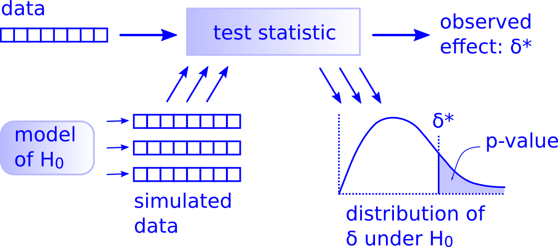
假设检验的目的在于，如果假设某一说法(零假设)为真，那么观测到与当前样本同样极端或更极端结果的概率有多大？

# 假设：平均杏仁重量等于3.6克，零假设为重量与3.6无显著差异，计算零假设为真时的统计量。
set.seed(1234)
null_dist <- almonds_sample_100 |>
  specify(response = weight) |>
  hypothesise(null = "point", mu = 3.6) |>
  generate(reps = 1000, type = "bootstrap") |>
  calculate(stat = "mean")
null_dist

Response: weight (numeric)
Null Hypothesis: point
# A tibble: 1,000 × 2
   replicate  stat
       <int> <dbl>
 1         1  3.56
 2         2  3.58
 3         3  3.56
 4         4  3.63
 5         5  3.62
 6         6  3.54
 7         7  3.59
 8         8  3.59
 9         9  3.60
10        10  3.59
# ℹ 990 more rows

# 计算p值
## 计算样本均值
x_bar_almonds <- almonds_sample_100 |>
  summarise(sample_mean = mean(weight)) |>
  select(sample_mean)
x_bar_almonds

# A tibble: 1 × 1
  sample_mean
        <dbl>
1        3.68

## 计算p值
null_dist |>
  get_p_value(obs_stat = x_bar_almonds, direction = "two sided")

# A tibble: 1 × 1
  p_value
    <dbl>
1   0.012

• p值小于0.05，因此拒绝零假设，认为平均杏仁重量不等于3.6克。

2.1.3 双因素方差分析

我们采用ggpubr宏包下的ToothGrowth来说明，这个数据集包含60个样本，记录着每10只豚鼠在不同的喂食方法和不同的药物剂量下，牙齿的生长情况.

• len : 牙齿长度
• supp : 两种喂食方法 (橙汁和维生素C)
• dose : 抗坏血酸剂量 (0.5, 1, and 2 mg)

library(ggpubr)
my_data <- ToothGrowth |>
  mutate(
    across(c(supp, dose), \(x) as.factor(x))
  )
my_data |>
  slice_head(n = 10)

    len supp dose
1   4.2   VC  0.5
2  11.5   VC  0.5
3   7.3   VC  0.5
4   5.8   VC  0.5
5   6.4   VC  0.5
6  10.0   VC  0.5
7  11.2   VC  0.5
8  11.2   VC  0.5
9   5.2   VC  0.5
10  7.0   VC  0.5

提出一个问题，不同喂食方法和不同药物剂量下，豚鼠牙齿长度的差异是否显著？这里是两个解释变量，所以问题需要双因素方差分析。

aov(len ~ supp + dose, data = my_data) |>
  broom::tidy()

# A tibble: 3 × 6
  term         df sumsq meansq statistic   p.value
  <chr>     <dbl> <dbl>  <dbl>     <dbl>     <dbl>
1 supp          1  205.  205.       14.0  4.29e- 4
2 dose          2 2426. 1213.       82.8  1.87e-17
3 Residuals    56  820.   14.7      NA   NA       

检验表明不同类型之间存在显著差异，但是并没有告诉我们具体谁与谁之间的不同。需要多重比较帮助我们解决这个问题。使用TurkeyHSD()函数。

aov(len ~ supp + dose, data = my_data) |>
  TukeyHSD(which = "dose") |>
  broom::tidy()

# A tibble: 3 × 7
  term  contrast null.value estimate conf.low conf.high adj.p.value
  <chr> <chr>         <dbl>    <dbl>    <dbl>     <dbl>       <dbl>
1 dose  1-0.5             0     9.13     6.22     12.0     1.32e- 9
2 dose  2-0.5             0    15.5     12.6      18.4     7.31e-12
3 dose  2-1               0     6.37     3.45      9.28    6.98e- 6

2.1.4 在tidyverse中进行方差分析

mtcars |>
  group_by(cyl) |>
  reframe(
    broom::tidy(aov(mpg ~ gear, data = cur_data()))
  ) |>
  select(term, statistic, p.value) |>
  filter(term != "Residuals") |>
  arrange(p.value)

# A tibble: 3 × 3
  term  statistic p.value
  <chr>     <dbl>   <dbl>
1 gear   1.17       0.308
2 gear   0.0297     0.866
3 gear   0.000451   0.984

2.2 infer包中的统计推断方法

我们回顾以下在infer包提供的一系列用于统计推断的函数，包括：

• specify()：通过公式的方式，指定结果变量和协变量（分组变量）。

• hypothesize()：指定specify()中选择的变量所要假设检验的类型，使用null参数(可以理解为”没有”假设，即零假设)，有三个选项

  • independence：适用于同时拥有响应变量和解释变量的情况，表明指定的响应变量和解释变量之间相互独立。也就是涉及两个样本的检验。
  • point：用于有响应变量的情况，它表明基于响应变量中的值所做出的点估计与某个参数相关。有时需要提供比例（p）、均值（mu）、中位数（med）或标准差（sigma）中的一个。也就是单个样本的检验。
  • paired independence：仅应用于已给出配对观测值之间预先计算好差值的响应变量。这表明配对值之间相减的顺序不会影响最终的分布。

• calculate()：计算指定的统计量。用参数stat="统计量"可以指定计算的统计量，具体可查看函数帮助。

• generate()：生成由specify()定义的模型的模拟分布。可以通过此函数定义重抽样方法（type），设定重复次数（rep）。其中，type参数有三种选项：

  • bootstrap：自助法，有放回的重抽样，常常对应hypothsize()中的null = "point"。
  • permute：置换法，无放回的抽样，常常对应hypothsize()中的null = "independence"。
  • draw：直接抽取，从hypothesize()中所制定的参数（p）的的理论分布中抽取样本，仅适用于单比例检验。

• 可以通过get_p_value()和get_ci()从前述计算结果中获取p值和置信区间；通过visualise()函数进行可视化，通过shade_p_value()函数在图形中添加p值，通过shade_ci()函数在图形中添加置信区间的阴影。

具体可参看 infer，以及ModernDive包的infer相关章节

2.3 统计检验与线性模型的等价性

对非统计专业的初学者（比如我）感觉 t-test， ANOVAs， Chi-Square test等太不友好了，每次用的时候，我都要去翻书看我用对了没有，还要担心p-value是否徘徊在0.05附近。或许，从t-test等统计检验方法开始学统计是个错误的开始。我们是不是应该更关心模型的理解，或者模型背后的理论呢。

常用的统计检验方法，如t-test，ANOVAs，Chi-Square test等，本质上都是线性模型。我认为，学习线性抹模型，掌握对模型的解释和理解，是更有价值的。

我们通过几个例子来说明统计检验和线性模型的等价性。

experim是一个模拟的数据集，这个虚拟的研究目的是，考察两种不同类型的干预措施对帮助学生应对即将到来的统计学课程的焦虑的影响。实验方案如下：

• 首先，学生完成一定数量的量表，包括对统计学课程的害怕(fost)，自信(confid)，抑郁(depress)指标。

• 然后，学生被等分成两组，组1 进行技能提升训练；组2进行信心提升训练。训练结束后，完成相同的量表。

• 三个月后，他们再次完成相同的量表。

• 即，相同的指标，在不同时期被测了3次，目的是考量不同类型的干预措施对指标的影响。

library(tidyverse)
edata <- read_csv(
  "D:/Document/0.Study R/0.NoteOfStudyR/datas/demo_data/experim.csv"
) |>
  mutate(group = if_else(group == "maths skills", 1, 2)) |>
  mutate(
    across(c(sex, id, group), as.factor)
  )
glimpse(edata)

Rows: 30
Columns: 18
$ id       <fct> 4, 10, 9, 3, 12, 11, 6, 5, 8, 13, 14, 1, 15, 7, 2, 27, 25, 19…
$ sex      <fct> male, male, male, male, male, male, male, male, male, male, m…
$ age      <dbl> 23, 21, 25, 30, 45, 22, 22, 26, 23, 21, 23, 19, 23, 19, 21, 2…
$ group    <fct> 2, 2, 1, 1, 2, 1, 2, 1, 2, 1, 2, 1, 1, 1, 2, 1, 1, 1, 2, 1, 1…
$ fost1    <dbl> 50, 47, 44, 47, 46, 39, 32, 44, 40, 47, 38, 32, 39, 36, 37, 4…
$ confid1  <dbl> 15, 14, 12, 11, 16, 13, 21, 17, 22, 20, 28, 20, 21, 24, 29, 1…
$ depress1 <dbl> 44, 42, 40, 43, 44, 43, 37, 46, 37, 50, 39, 44, 47, 38, 50, 4…
$ fost2    <dbl> 48, 45, 39, 42, 45, 40, 33, 37, 40, 45, 37, 28, 35, 32, 36, 4…
$ confid2  <dbl> 16, 15, 18, 16, 16, 20, 22, 20, 23, 25, 27, 25, 26, 28, 30, 1…
$ depress2 <dbl> 44, 42, 40, 43, 45, 42, 36, 47, 37, 48, 36, 43, 47, 35, 47, 4…
$ fost3    <dbl> 45, 44, 36, 41, 43, 39, 32, 32, 40, 46, 32, 23, 35, 30, 34, 3…
$ confid3  <dbl> 14, 18, 19, 20, 20, 22, 23, 26, 26, 27, 29, 30, 30, 32, 34, 1…
$ depress3 <dbl> 40, 40, 38, 43, 43, 38, 35, 42, 35, 46, 34, 40, 47, 35, 45, 4…
$ exam     <dbl> 52, 55, 58, 60, 58, 62, 59, 70, 60, 70, 72, 82, 79, 80, 90, 5…
$ mah_1    <dbl> 0.5699842, 1.6594031, 3.5404715, 2.4542143, 0.9443036, 1.6257…
$ DepT1gp2 <chr> "not depressed", "not depressed", "not depressed", "not depre…
$ DepT2Gp2 <chr> "not depressed", "not depressed", "not depressed", "not depre…
$ DepT3gp2 <chr> "not depressed", "not depressed", "not depressed", "not depre…

2.3.1 t检验和线性回归的比较

我们想检验第一次测量的抑郁指标得分（depress1）的分布，是否明显偏离正态分布（均值为0）。那么：

• 零假设应为第一次测量的抑郁指标得分（depress1）的分布服从正态分布，均值为0.
• 备择假设为第一次测量的抑郁指标得分（depress1）的分布不服从正态分布，均值不为0。

model_1_t <- t.test(edata$depress1, data = edata)
model_1_t

    One Sample t-test

data:  edata$depress1
t = 50.734, df = 29, p-value < 2.2e-16
alternative hypothesis: true mean is not equal to 0
95 percent confidence interval:
 40.81871 44.24796
sample estimates:
mean of x 
 42.53333 

输出结果显示，p值非常小（接近于0），应拒绝零假设，即第一次测量的抑郁指标得分（depress1）的分布不服从正态分布，均值为0。

那么我们再用线性回归的方法来做一次。[depress1 ~ 1，意为用截距预测响应变量，也可看做是检验响应变量的均值是否显著偏离0.]

model_1_lm <- lm(depress1 ~ 1, data = edata)
summary(model_1_lm)

Call:
lm(formula = depress1 ~ 1, data = edata)

Residuals:
    Min      1Q  Median      3Q     Max 
-9.5333 -3.5333  0.4667  2.4667  7.4667 

Coefficients:
            Estimate Std. Error t value Pr(>|t|)    
(Intercept)  42.5333     0.8384   50.73   <2e-16 ***
---
Signif. codes:  0 '***' 0.001 '**' 0.01 '*' 0.05 '.' 0.1 ' ' 1

Residual standard error: 4.592 on 29 degrees of freedom

将两种方法的结果规整在一起以方便比较

library(broom)
model_1_t_tidy <- tidy(model_1_t) |> mutate(model = "t.test(y)")
model_1_lm_tidy <- tidy(model_1_lm) |> mutate(model = "lm(y ~ 1)")

bind_rows(model_1_lm_tidy, model_1_t_tidy) |>
  select(model, estimate, statistic, p.value)

# A tibble: 2 × 4
  model     estimate statistic  p.value
  <chr>        <dbl>     <dbl>    <dbl>
1 lm(y ~ 1)     42.5      50.7 7.07e-30
2 t.test(y)     42.5      50.7 7.07e-30

输出的结果完全一致！

其他诸如关联、单因素方差分析、双因素方差分析等与线性模型的对比，可参看 这篇文章。

因此，相比于做统计检验，线性模型其实更好，因为lm()不仅给出了变量作为整体是否对响应变量产生影响外，还提供了更多因子之间的信息。

2.4 案例1：音乐热度动态分析-metal music是否比 deep house music 更受欢迎？

使用spotify_by_genre数据集探索metal music和deep house music的热度动态。这个数据集包含在moderndive包中。

2.4.1 p值

# load data and EDA
spotify_metal_deephouse <- moderndive::spotify_by_genre |>
  filter(track_genre %in% c("metal", "deep-house")) |>
  select(track_genre, artists, track_name, popularity, popular_or_not)
spotify_metal_deephouse |>
  group_by(track_genre, popular_or_not) |>
  summarize(
    n = n(), # same as tally()
    prop = n / 1000
  )

# A tibble: 4 × 4
# Groups:   track_genre [2]
  track_genre popular_or_not     n  prop
  <chr>       <chr>          <int> <dbl>
1 deep-house  not popular      471 0.471
2 deep-house  popular          529 0.529
3 metal       not popular      437 0.437
4 metal       popular          563 0.563

## plot
ggplot(spotify_metal_deephouse, aes(x = track_genre, fill = popular_or_not)) +
  geom_bar() +
  labs(x = "Genre of track")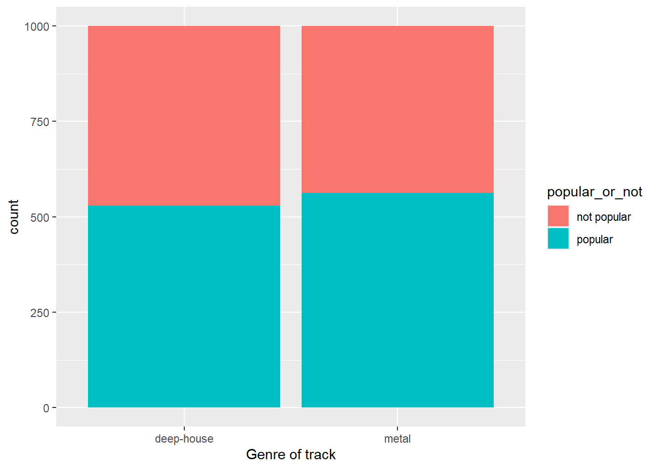

# conducting hypothesis test
null_distribution <- spotify_metal_deephouse |>
  specify(formula = popular_or_not ~ track_genre, success = "popular") |>
  hypothesise(null = "independence") |>
  generate(reps = 1000, type = "permute") |>
  calculate(stat = "diff in props", order = c("metal", "deep-house"))
## calculate difference stat of observed data withour hypothesis() and generate()
obs_diff_prop <- spotify_metal_deephouse |>
  specify(formula = popular_or_not ~ track_genre, success = "popular") |>
  calculate(stat = "diff in props", order = c("metal", "deep-house"))
obs_diff_prop

Response: popular_or_not (factor)
Explanatory: track_genre (factor)
# A tibble: 1 × 1
    stat
   <dbl>
1 0.0340

## calculate p-value
### plot
visualize(null_distribution, bins = 25) +
  shade_p_value(obs_stat = obs_diff_prop, direction = "right")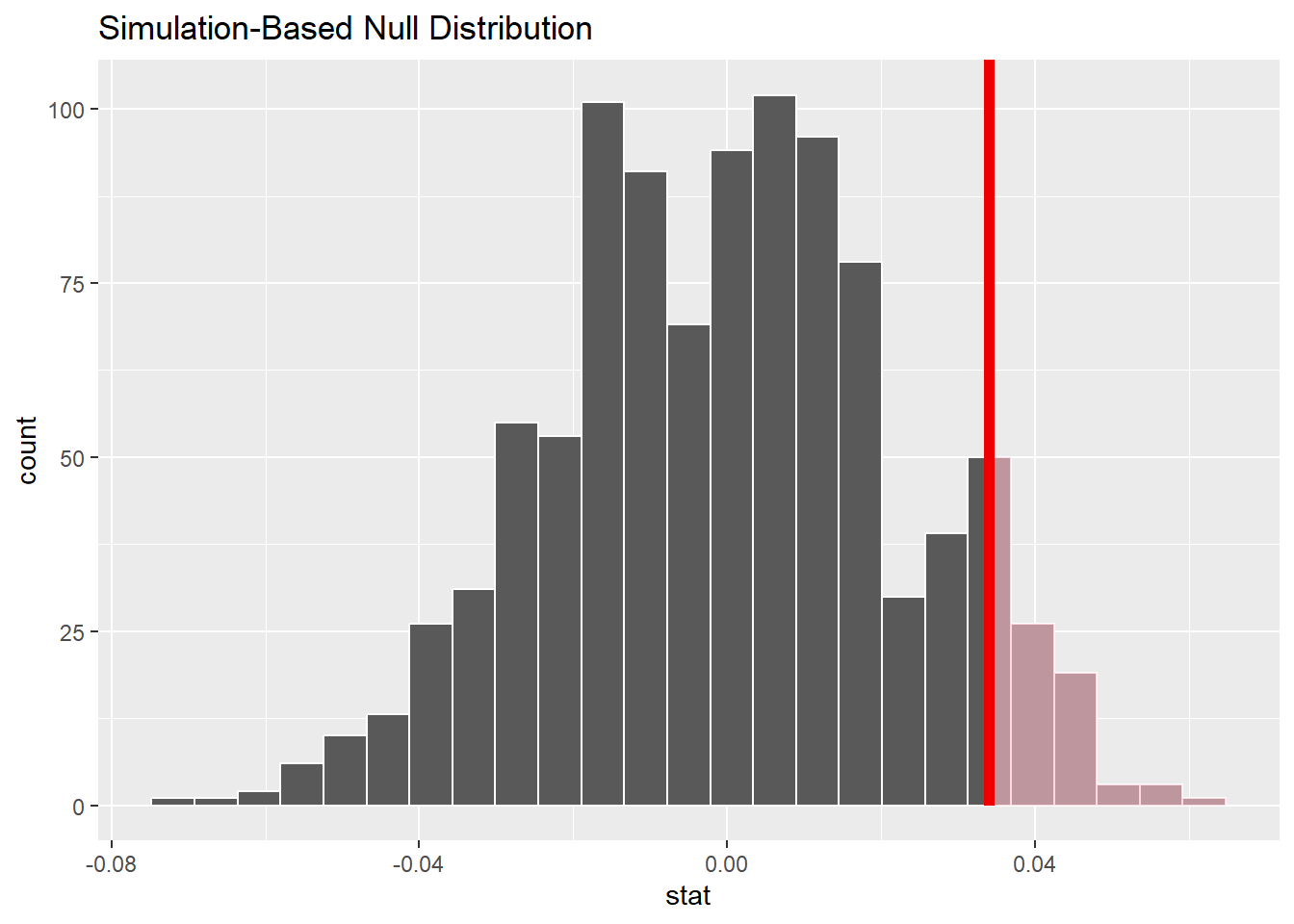

### get p-value
null_distribution |>
  get_p_value(obs_stat = obs_diff_prop, direction = "right")

# A tibble: 1 × 1
  p_value
    <dbl>
1   0.083

• p值图中，直方图为零假设的分布。
• 红色的实线为观察值的检验统计量，也就是真实数据集的样本差异。
• 直方图的阴影区域为p值，即在零假设为真的情况下，获得与观察到的检验统计量相同或更极端的检验统计量的概率，换句话说，阴影部分就是零假设为真时的概率。

2.4.2 置信区间

bootstrap_distribution <- spotify_metal_deephouse |>
  specify(formula = popular_or_not ~ track_genre, success = "popular") |>
  # Change 1 - Remove hypothesize():
  # hypothesize(null = "independence") |>
  # Change 2 - Switch type from "permute" to "bootstrap":
  generate(reps = 1000, type = "bootstrap") |>
  calculate(stat = "diff in props", order = c("metal", "deep-house"))
percentile_ci <- bootstrap_distribution |>
  get_ci(level = 0.90, type = "percentile")
percentile_ci

# A tibble: 1 × 2
  lower_ci upper_ci
     <dbl>    <dbl>
1 -0.00333   0.0723

# plot
visualise(bootstrap_distribution) +
  shade_ci(endpoints = percentile_ci)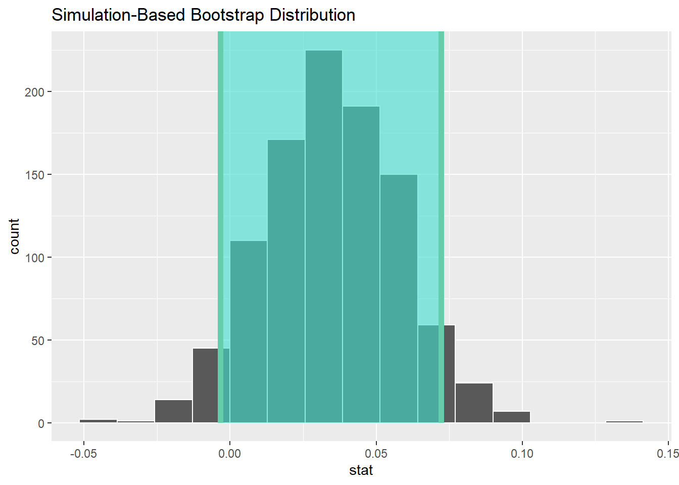

• 置信区间总体都是大于0值的，换句话说，参与比较的两个变量是显著不同的。

2.5 案例2：电影评分高低

以下是关于电影评分的数据集，包含58788 行 和 24 变量，我们想了解爱情片与动作片的平均得分是否显著不同。

如果使用传统的t检验方法，则需要先设定假设，然后进行统计检验：

1. 设定假设：

再次强调，零假设是我们希望证实的事件的对立事件，即我们希望证实为假的事件。

• \(H_0: \mu_1 = \mu_2\)，即爱情片与动作片的平均得分没有显著不同。
• \(H_1: \mu_1 \neq \mu_2\)，即爱情片与动作片的平均得分有显著不同。

2. 进行统计检验：t.test()，观察p值等结果推断是否拒绝零假设。

本章我们主要使用infer包进行抽样和推断。

统计推断基本框架

2.5.1 数据准备和简单EDA

d <- ggplot2movies::movies
# basic data cleaning
movies_genre_sample <- d |>
  select(title, year, rating, Action, Romance) |>
  filter(!(Action == 1 & Romance == 1)) |> # remove movies with both Action and Romance
  mutate(
    genre = case_when(
      Action == 1 ~ "Action",
      Romance == 1 ~ "Romance",
      TRUE ~ "Neither"
    )
  ) |>
  filter(genre != "Neither") |>
  select(-Action, -Romance) |>
  group_by(genre) |>
  # slice_sample(n = 34)  |>   # select 34 movies for each genre
  slice_head(n = 34) |>
  ungroup()
movies_genre_sample

# A tibble: 68 × 4
   title                     year rating genre 
   <chr>                    <int>  <dbl> <chr> 
 1 $windle                   2002    5.3 Action
 2 'A' gai waak              1983    7.1 Action
 3 'A' gai waak juk jaap     1987    7.2 Action
 4 'Crocodile' Dundee II     1988    5   Action
 5 'Gator Bait               1974    3.5 Action
 6 'Sheba, Baby'             1975    5.5 Action
 7 ...Po prozvishchu 'Zver'  1990    4.7 Action
 8 ...tick...tick...tick...  1970    6   Action
 9 002 agenti segretissimi   1964    3.6 Action
10 10 Magnificent Killers    1977    2.6 Action
# ℹ 58 more rows

# boxplot
ggplot(movies_genre_sample, aes(x = genre, y = rating)) +
  geom_boxplot() +
  geom_jitter()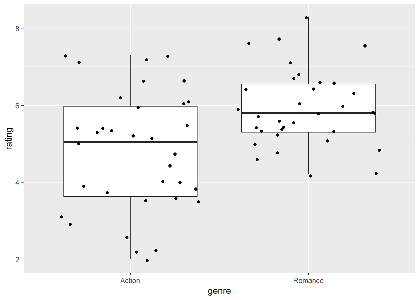

# dis-plot
ggplot(movies_genre_sample, aes(x = rating)) +
  geom_histogram(binwidth = 1, color = "white") +
  facet_grid(vars(genre))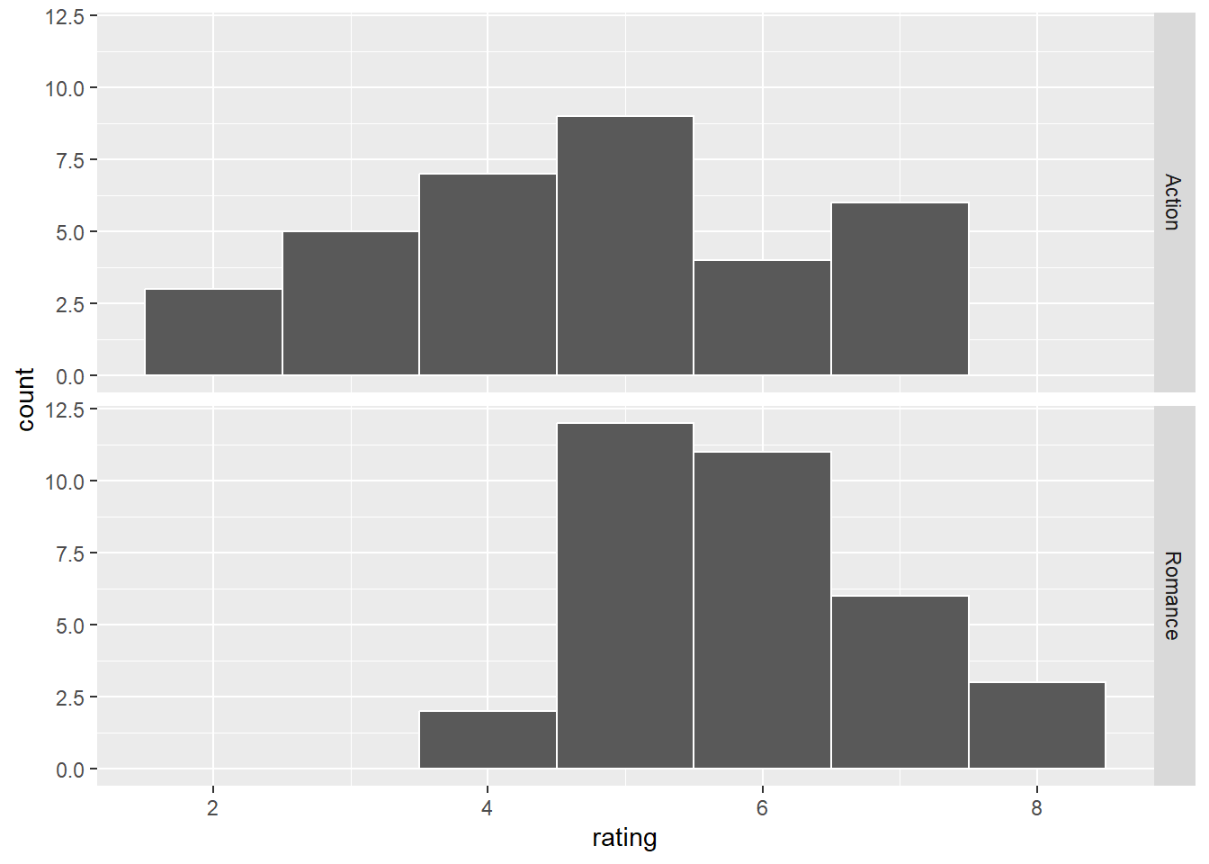

# mean rating of action and romance movies
movies_genre_sample |>
  group_by(genre) |>
  summarize(
    mean_rating = mean(rating),
    std_dev = sd(rating),
    n = n()
  )

# A tibble: 2 × 4
  genre   mean_rating std_dev     n
  <chr>         <dbl>   <dbl> <int>
1 Action         4.78   1.56     34
2 Romance        5.91   0.994    34

2.5.2 基于infer的模拟检验

library(infer)

set.seed(1234)

# calculate observed difference in means
obs_diff <- movies_genre_sample |>
  specify(formula = rating ~ genre) |>
  calculate(
    stat = "diff in means",
    order = c("Romance", "Action")
  )
obs_diff

Response: rating (numeric)
Explanatory: genre (factor)
# A tibble: 1 × 1
   stat
  <dbl>
1  1.12

# statistical inference
null_dist <- movies_genre_sample |>
  specify(formula = rating ~ genre) |>
  hypothesize(null = "independence") |>
  generate(reps = 5000, type = "permute") |>
  calculate(
    stat = "diff in means",
    order = c("Romance", "Action")
  )
head(null_dist)

Response: rating (numeric)
Explanatory: genre (factor)
Null Hypothesis: indep...
# A tibble: 6 × 2
  replicate    stat
      <int>   <dbl>
1         1  0.476 
2         2  0.565 
3         3  0.335 
4         4  0.188 
5         5 -0.0412
6         6 -0.265 

## visualize the null distribution
null_dist |>
  visualise() +
  shade_p_value(obs_stat = obs_diff, direction = "both")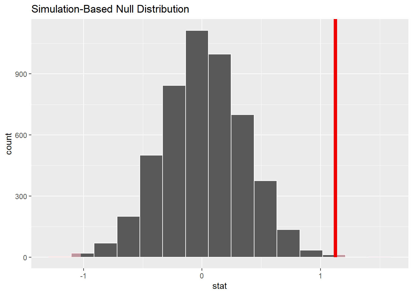

## calculate p-value
p_value <- null_dist |>
  get_p_value(obs_stat = obs_diff, direction = "both")
p_value

# A tibble: 1 × 1
  p_value
    <dbl>
1  0.0024

• \(p_value = 0.0028 < 0.05\)。
• 因此，我们拒绝零假设，认为爱情片与动作片的平均得分在95%的置信水平上有显著差异，担当置信水平为99%(\(alpha = 0.001\))时差异性不显著。
• 由平均值计算结果可得，动作电影的评分比爱情电影更低。

2.6 案例3：航天事业的预算是否有党派或门户之见

# load data
gss <- read_rds("./data/gss.rds")
gss |>
  select(NASA, party) |>
  count(NASA, party) |>
  head(5)

# A tibble: 5 × 3
  NASA        party     n
  <fct>       <fct> <int>
1 TOO LITTLE  Dem       8
2 TOO LITTLE  Ind      13
3 TOO LITTLE  Rep       9
4 ABOUT RIGHT Dem      22
5 ABOUT RIGHT Ind      37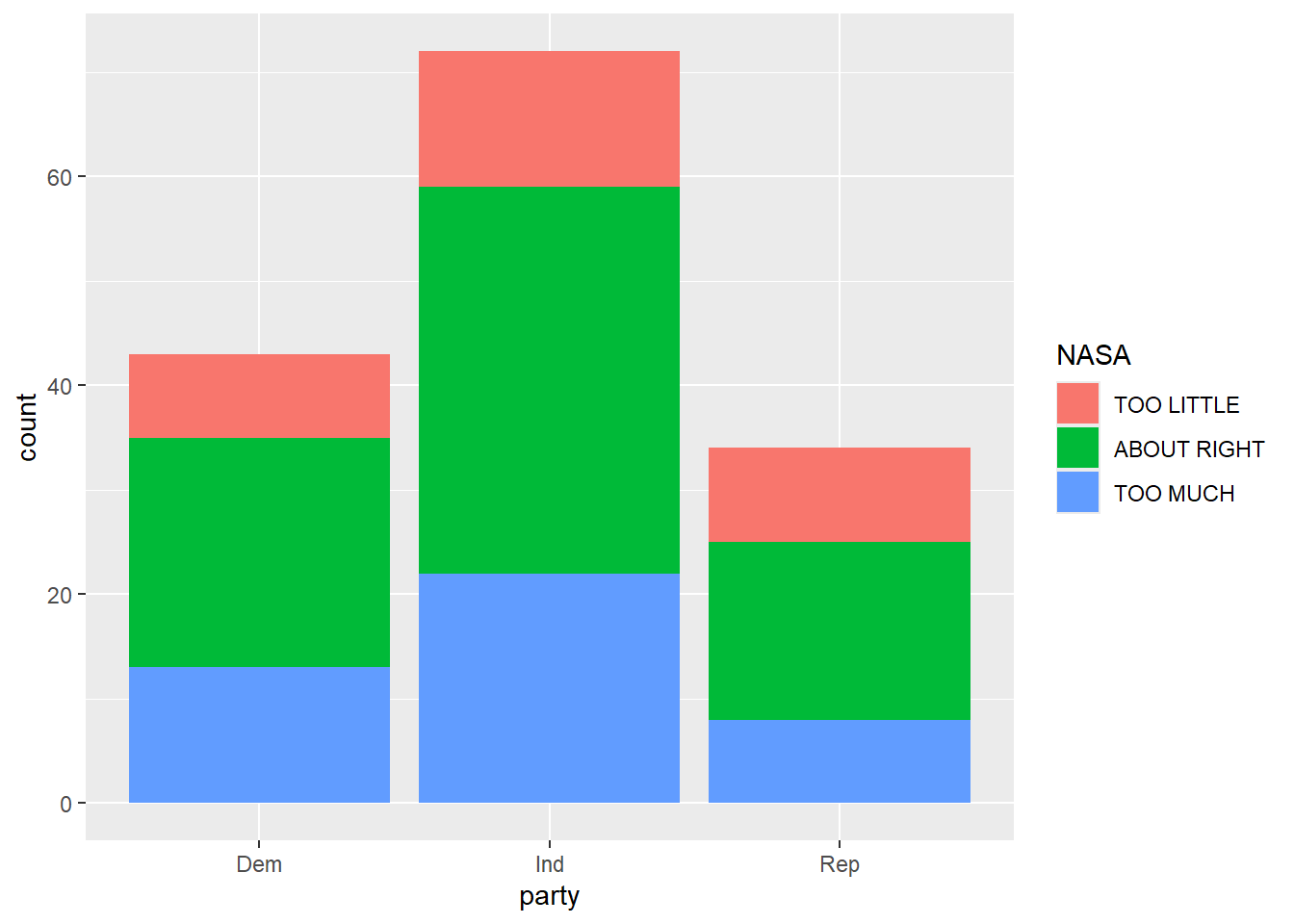

# EDA-plot
ggplot(gss, aes(x = party, fill = NASA)) +
  geom_bar()

假设： - \(H_0\)，即党派与非党派的预算没有显著不同。 - \(H_1\)，即党派的预算显著大于非党派的预算。

2.6.1 基于infer的模拟检验

# calculate observed difference in means
set.seed(1234)
obs_stat <- gss |>
  specify(NASA ~ party) |>
  calculate(stat = "Chisq") # calculate Chisq test statistic
obs_stat

Response: NASA (factor)
Explanatory: party (factor)
# A tibble: 1 × 1
   stat
  <dbl>
1  1.33

# statistical inference
null_dist <- gss |>
  specify(NASA ~ party) |>
  hypothesise(null = "independence") |>
  generate(reps = 5000, type = "permute") |> # 置换法重抽样
  calculate(stat = "Chisq")
null_dist

Response: NASA (factor)
Explanatory: party (factor)
Null Hypothesis: independence
# A tibble: 5,000 × 2
   replicate  stat
       <int> <dbl>
 1         1  8.67
 2         2  3.43
 3         3  1.43
 4         4  4.49
 5         5  3.50
 6         6  3.07
 7         7  5.77
 8         8  3.86
 9         9  1.97
10        10  7.87
# ℹ 4,990 more rows

# plot
null_dist |>
  visualise() +
  shade_p_value(obs_stat = obs_stat, direction = "right")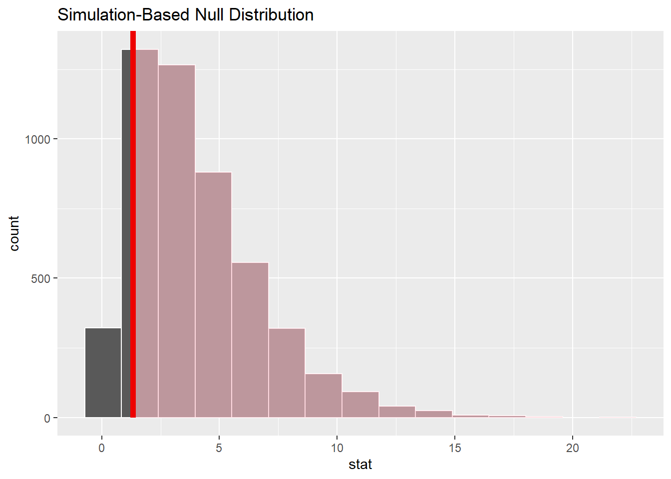

# get p-value
null_dist |>
  get_p_value(obs_stat = obs_stat, direction = "right")

# A tibble: 1 × 1
  p_value
    <dbl>
1   0.860

• 结果显示 p_value > 0.05，不能拒绝 H0，我们没有足够的证据证明党派之间有显著差异。

2.7 案例4：原住民中女学生多？

案例 quine 数据集有 146 行 5 列，包含学生的生源、文化、性别和学习成效，具体说明如下

• Eth: 民族背景：原住民与否 (是”A”; 否 “N”)
• Sex: 性别
• Age: 年龄组 (“F0”, “F1,” “F2” or “F3”)
• Lrn: 学习者状态(平均水平 “AL”， 学习缓慢 “SL”)
• Days：一年中缺勤天数

假设： - \(H_0\)，即原住民中女学生少。 - \(H_1\)，即原住民中女学生多。

# load data
td <- MASS::quine |>
  as_tibble() |>
  mutate(
    across(c(Sex, Eth), as_factor)
  )
td

# A tibble: 146 × 5
   Eth   Sex   Age   Lrn    Days
   <fct> <fct> <fct> <fct> <int>
 1 A     M     F0    SL        2
 2 A     M     F0    SL       11
 3 A     M     F0    SL       14
 4 A     M     F0    AL        5
 5 A     M     F0    AL        5
 6 A     M     F0    AL       13
 7 A     M     F0    AL       20
 8 A     M     F0    AL       22
 9 A     M     F1    SL        6
10 A     M     F1    SL        6
# ℹ 136 more rows

# EDA-count Eth and Sex
td |>
  count(Eth, Sex)

# A tibble: 4 × 3
  Eth   Sex       n
  <fct> <fct> <int>
1 A     F        38
2 A     M        31
3 N     F        42
4 N     M        35

2.7.0.1 基于infer的模拟检验

set.seed(1234)
obs_diff <- td |>
  specify(Sex ~ Eth, success = "F") |>
  calculate(
    stat = "diff in props",
    order = c("A", "N")
  )
obs_diff

Response: Sex (factor)
Explanatory: Eth (factor)
# A tibble: 1 × 1
     stat
    <dbl>
1 0.00527

# statistical inference
null_dist <- td |>
  specify(Sex ~ Eth, success = "F") |>
  hypothesize(null = "independence") |>
  generate(reps = 5000, type = "permute") |>
  calculate(
    stat = "diff in props",
    order = c("A", "N")
  )
null_dist

Response: Sex (factor)
Explanatory: Eth (factor)
Null Hypothesis: independence
# A tibble: 5,000 × 2
   replicate     stat
       <int>    <dbl>
 1         1  0.00527
 2         2 -0.187  
 3         3 -0.0772 
 4         4 -0.0222 
 5         5 -0.0222 
 6         6  0.0602 
 7         7  0.0602 
 8         8 -0.0772 
 9         9  0.00527
10        10 -0.132  
# ℹ 4,990 more rows

# plot
null_dist |>
  visualise() +
  shade_p_value(obs_stat = obs_diff, direction = "left")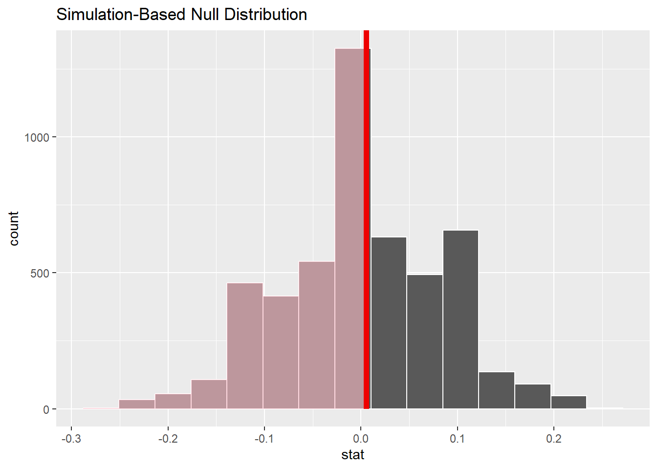

# get p-value
null_dist |>
  get_p_value(obs_stat = obs_diff, direction = "left")

# A tibble: 1 × 1
  p_value
    <dbl>
1   0.589

# get confidence interval
null_dist |>
  get_ci(level = 0.95, type = "percentile")

# A tibble: 1 × 2
  lower_ci upper_ci
     <dbl>    <dbl>
1   -0.160    0.170

• \(p_value = 1 >> 0.05\)，不能拒绝 \(H_0\)，我们没有足够的证据证明原住民中女学生多。
• 95%的置信区间为[-0.16, 0.17]。

---

1. 这是R语言的基本语法，infer包有更贴合tidyverse风格的统计推断函数，具体可参看inferd的官方文档。。