tidymodels::tidymodels_prefer()

basic_rec <- recipe(
  Sale_Price ~ Neighborhood + Gr_Liv_Area + Year_Built + Bldg_Type + Latitude + Longitude,
  data = ames_train
) %>%
  step_log(Gr_Liv_Area, base = 10) %>%
  step_other(Neighborhood, threshold = 0.01) %>%
  step_dummy(all_nominal_predictors())

interaction_rec <- basic_rec %>%
  step_interact(~ Gr_Liv_Area:starts_with("Bldg_Type_"))

spline_rec <- interaction_rec %>%
  step_ns(Latitude, Longitude, deg_free = 20)

preproc <- list(
  basic = basic_rec,
  interaction = interaction_rec,
  spline = spline_rec
)

lm_wflows <- workflow_set(
  preproc = preproc,
  model = list(lm = linear_reg()),
  cross = FALSE
)10 通过重采样比较模型
10.1 使用workflowset创建多个模型
在 Section 6.3.2 中展示了如何使用workflowset创建多个模型。在本节中,我们将展示如何使用workflowset比较多个模型。具体的思路为:
- 创建数个不同的线性模型。
- 每个模型使用不同的预处理步骤,以测试不同预处理是否可以改善模型表现。
- 将这些预处理步骤组合为一个
workflowset。
接下来我们需要对每一个模型轮流进行重抽样评估,需要使用一个类似于purrr风格的函数,为workflow_map():
- 该函数的第一个参数是一个可以用于workflow的函数名称(注意,这个名称需要用引号扩起来),随后是该函数的选项。
- 同时可以设置
verbose和seed参数,确保每个模型使用与其他模型相同的随机数种子。
lm_models_res <- lm_wflows %>%
  workflow_map(
    "fit_resamples",
    # fit_resamples()选项
    resamples = ames_folds, control = keep_pred,
    # workflow_map()选项
    seed = 1001, verbose = TRUE
  )
lm_models_res
# A workflow set/tibble: 3 × 4
wflow_id info option result
<chr> <list> <list> <list>
1 basic_lm <tibble [1 × 4]> <opts[2]> <rsmp[+]>
2 interaction_lm <tibble [1 × 4]> <opts[2]> <rsmp[+]>
3 spline_lm <tibble [1 × 4]> <opts[2]> <rsmp[+]># 提取性能指标
collect_metrics(lm_models_res) %>%
filter(.metric == "rmse")# A tibble: 3 × 9
wflow_id .config preproc model .metric .estimator mean n std_err
<chr> <chr> <chr> <chr> <chr> <chr> <dbl> <int> <dbl>
1 basic_lm pre0_mod… recipe line… rmse standard 0.0803 10 0.00264
2 interaction_lm pre0_mod… recipe line… rmse standard 0.0799 10 0.00272
3 spline_lm pre0_mod… recipe line… rmse standard 0.0784 10 0.00283以上的代码创建了三个不同的模型,每个模型都使用不同的预处理步骤。然后使用workflow_map()函数对每个模型进行重抽样评估,并使用collect_metrics()函数提取性能指标。
如果我们希望在workflowset中在增加其他需要比较的模型,只需要将需要增加的模型转换为一个workflowset对象,并添加到原先的workflowset中即可。
four_models_res <-
  as_workflow_set(random_forest = rf_res) %>%
  bind_rows(lm_models_res)
four_models_res %>%
  collect_metrics() %>%
  filter(.metric == "rmse")
# A tibble: 4 × 9
wflow_id .config preproc model .metric .estimator mean n std_err
<chr> <chr> <chr> <chr> <chr> <chr> <dbl> <int> <dbl>
1 random_forest pre0_mod… formula rand… rmse standard 0.0720 10 0.00306
2 basic_lm pre0_mod… recipe line… rmse standard 0.0803 10 0.00264
3 interaction_lm pre0_mod… recipe line… rmse standard 0.0799 10 0.00272
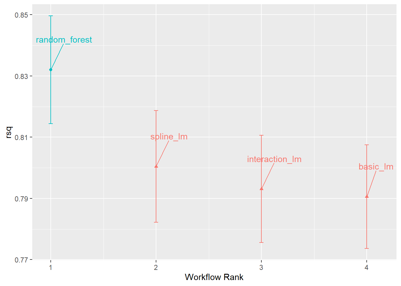
4 spline_lm pre0_mod… recipe line… rmse standard 0.0784 10 0.00283现在,4个模型中每一个都有10个重抽样的性能估计,这些指标都可用来进行模型之间的比较。
10.1.1 可视化模型之间的比较
10.2 比较重抽样得到的性能指标
不同重抽样间的结果往往不同,某个在一些重抽样中,表现很好的模型,在其他重抽样中可能表现很差。因此,我们需要比较不同模型在不同重抽样中的性能表现。
这个现象被称为重抽样间的变异性
我们通过上节已经拟合的4个模型中的 \(r^2\) 值来说明这个问题。
rsq_indiv_estimates <- four_models_res %>%
  collect_metrics(summarize = FALSE) %>%
  filter(.metric == "rsq")

# 转换为宽数据
rsq_wide <- rsq_indiv_estimates %>%
  pivot_wider(
    id_cols = "id", names_from = "wflow_id", values_from = ".estimate"
  )
# 计算相关系数
corrr::correlate(rsq_wide %>% select(-id), quiet = TRUE)
# A tibble: 4 × 5
term random_forest basic_lm interaction_lm spline_lm
<chr> <dbl> <dbl> <dbl> <dbl>
1 random_forest NA 0.887 0.887 0.891
2 basic_lm 0.887 NA 0.993 0.989
3 interaction_lm 0.887 0.993 NA 0.984
4 spline_lm 0.891 0.989 0.984 NA 可以看到,不同模型之间的相关性很高,这表明在不同模型间存在较大的重抽样内相关性。
所以在模型比较或查看重抽样结果之前,最好先定义一个相关的实际效应量(practical effect size)。这个实际效应量可以帮助我们确定模型之间的差异是否具有实际意义。例如,在本例中我们可以认定如果两个模型的\(R^2\)相差不超过\(\pm2\%\),可认为两个模型没有实际的差别,这种情况下,小于2%的差异即使显著,也不重要。