3 用数据讲故事

library(tidyverse)
library(scales)
library(moderndive)
library(infer)
library(gridExtra)
library(GGally)
library(ggrepel)
library(patchwork)

3.1 西雅图房价-案例研究1

我们将创建一个多元回归模型来预测西雅图的房价。

结果变量(y)为数据中的price列。
预测变量(x)为数据中的sqft_living数值列和condition分类列。分别表示房屋面积和房屋状况。

3.1.1 EDA

EDA是数据分析的第一步，目的是了解数据的基本情况和特征。

常见的EDA步骤包括：

查看原始数据的结构和变量信息。
计算描述性统计量，如均值、中位数、标准差、各种分位数等。使用moderndive包中的tidy_summary()函数可以轻松计算这些统计量。
可视化数据分布和关系，如直方图、散点图、箱线图等。
多变量可视化，探究多个变量之间的关系。

在执行以上步骤后，根据结果可以问自己以下几个问题：

哪些变量是数值型的？哪些是分类型的？
对于分类型变量，它们的水平是什么？
除了我们将在回归模型中使用的变量之外，还有哪些变量在预测房价的模型中会有用？

# 查看数据基本信息
glimpse(house_prices)

Rows: 21,613
Columns: 21
$ id            <chr> "7129300520", "6414100192", "5631500400", "2487200875", …
$ date          <date> 2014-10-13, 2014-12-09, 2015-02-25, 2014-12-09, 2015-02…
$ price         <dbl> 221900, 538000, 180000, 604000, 510000, 1225000, 257500,…
$ bedrooms      <int> 3, 3, 2, 4, 3, 4, 3, 3, 3, 3, 3, 2, 3, 3, 5, 4, 3, 4, 2,…
$ bathrooms     <dbl> 1.00, 2.25, 1.00, 3.00, 2.00, 4.50, 2.25, 1.50, 1.00, 2.…
$ sqft_living   <int> 1180, 2570, 770, 1960, 1680, 5420, 1715, 1060, 1780, 189…
$ sqft_lot      <int> 5650, 7242, 10000, 5000, 8080, 101930, 6819, 9711, 7470,…
$ floors        <dbl> 1.0, 2.0, 1.0, 1.0, 1.0, 1.0, 2.0, 1.0, 1.0, 2.0, 1.0, 1…
$ waterfront    <lgl> FALSE, FALSE, FALSE, FALSE, FALSE, FALSE, FALSE, FALSE, …
$ view          <int> 0, 0, 0, 0, 0, 0, 0, 0, 0, 0, 0, 0, 0, 0, 0, 3, 0, 0, 0,…
$ condition     <fct> 3, 3, 3, 5, 3, 3, 3, 3, 3, 3, 3, 4, 4, 4, 3, 3, 3, 4, 4,…
$ grade         <fct> 7, 7, 6, 7, 8, 11, 7, 7, 7, 7, 8, 7, 7, 7, 7, 9, 7, 7, 7…
$ sqft_above    <int> 1180, 2170, 770, 1050, 1680, 3890, 1715, 1060, 1050, 189…
$ sqft_basement <int> 0, 400, 0, 910, 0, 1530, 0, 0, 730, 0, 1700, 300, 0, 0, …
$ yr_built      <int> 1955, 1951, 1933, 1965, 1987, 2001, 1995, 1963, 1960, 20…
$ yr_renovated  <int> 0, 1991, 0, 0, 0, 0, 0, 0, 0, 0, 0, 0, 0, 0, 0, 0, 0, 0,…
$ zipcode       <fct> 98178, 98125, 98028, 98136, 98074, 98053, 98003, 98198, …
$ lat           <dbl> 47.5112, 47.7210, 47.7379, 47.5208, 47.6168, 47.6561, 47…
$ long          <dbl> -122.257, -122.319, -122.233, -122.393, -122.045, -122.0…
$ sqft_living15 <int> 1340, 1690, 2720, 1360, 1800, 4760, 2238, 1650, 1780, 23…
$ sqft_lot15    <int> 5650, 7639, 8062, 5000, 7503, 101930, 6819, 9711, 8113, …

# 计算统计量
house_prices |>
  select(price, sqft_living, condition) |>
  tidy_summary()

# A tibble: 7 × 11
  column        n group type    min     Q1    mean median     Q3     max      sd
  <chr>     <int> <chr> <chr> <dbl>  <dbl>   <dbl>  <dbl>  <dbl>   <dbl>   <dbl>
1 price     21613 <NA>  nume… 75000 321950 540088. 450000 645000 7700000 367127.
2 sqft_liv… 21613 <NA>  nume…   290   1427   2080.   1910   2550   13540    918.
3 condition    30 1     fact…    NA     NA     NA      NA     NA      NA     NA 
4 condition   172 2     fact…    NA     NA     NA      NA     NA      NA     NA 
5 condition 14031 3     fact…    NA     NA     NA      NA     NA      NA     NA 
6 condition  5679 4     fact…    NA     NA     NA      NA     NA      NA     NA 
7 condition  1701 5     fact…    NA     NA     NA      NA     NA      NA     NA

# 可视化
## hisatogram of house price
p1 <- ggplot(house_prices, aes(x = price)) +
  geom_histogram(color = "white") +
  labs(x = "price (USD)", title = "House price")
## Histogram of sqft_living:
p2 <- ggplot(house_prices, aes(x = sqft_living)) +
  geom_histogram(color = "white") +
  labs(x = "living space (square feet)", title = "House size")
## Barplot of condition:
p3 <- ggplot(house_prices, aes(x = condition)) +
  geom_bar() +
  labs(x = "condition", title = "House condition")

p1 / p2 / p3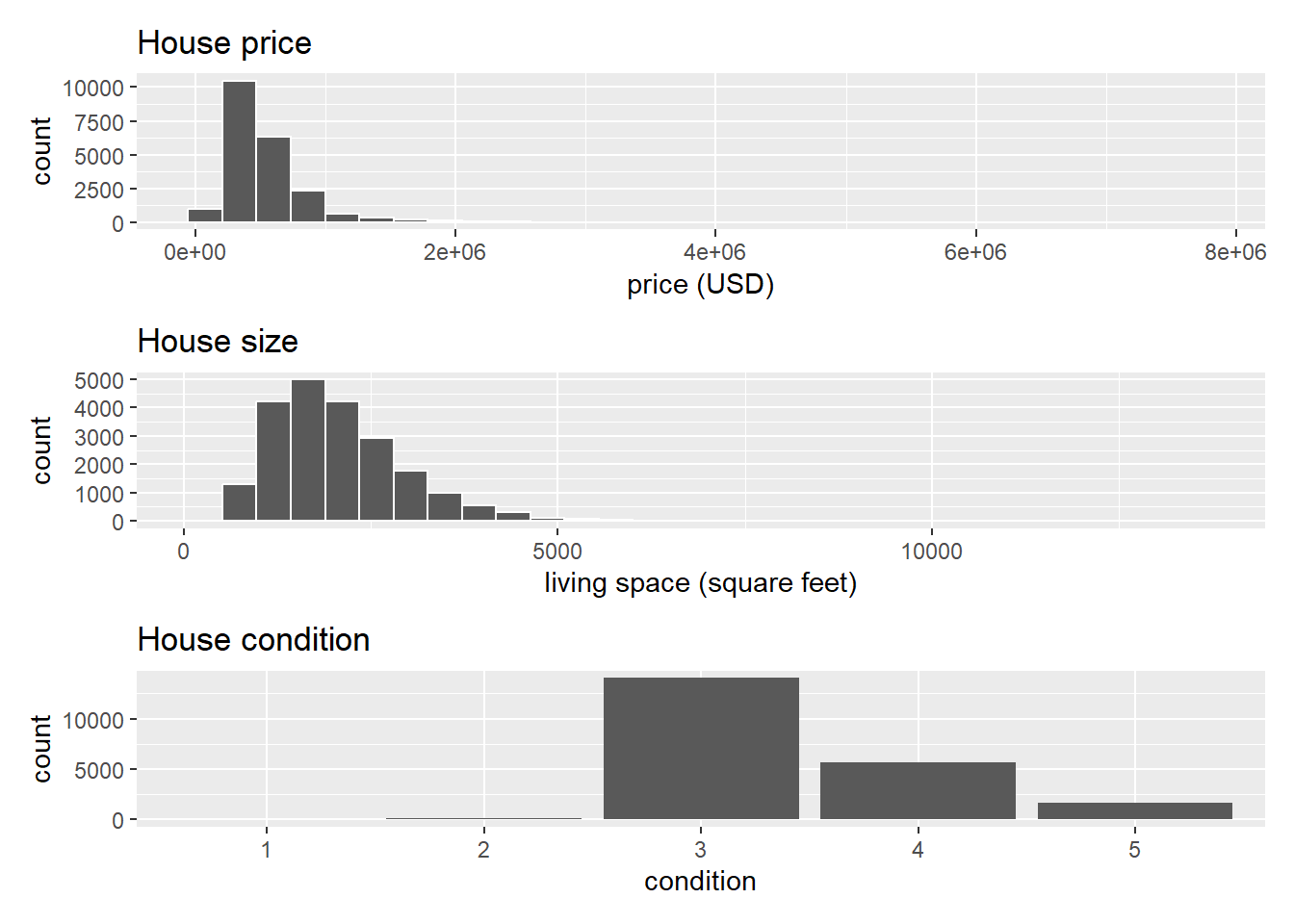

大多数房屋的condition为3，1和2的几乎没有。
大多数房屋的price低于200万美元，但也有极少数房屋的价格接近800万美元。变量price呈右偏分布，表现为长长的右尾。
大多数房屋的居住面积似乎不足5000平方英尺，此外该变量也呈右偏分布，尽管不像price变量那样显著。
针对两个变量的偏向分布情况，可以对其使用对数变换来消除。*注意，在后续进行多元回归建模时，也要使用对数变换后的变量。

# log conversion
house_prices_log <- house_prices |>
  mutate(log10_price = log10(price), log10_size = log10(sqft_living)) |>
  select(log10_price, log10_size, condition)

# multiple var plot
ggplot(
  house_prices_log,
  aes(x = log10_size, y = log10_price, col = condition)
) +
  geom_point(alpha = 0.05) +
  geom_smooth(method = "lm", se = FALSE) +
  labs(y = "log10 price", x = "log10 size", title = "House prices in Seattle")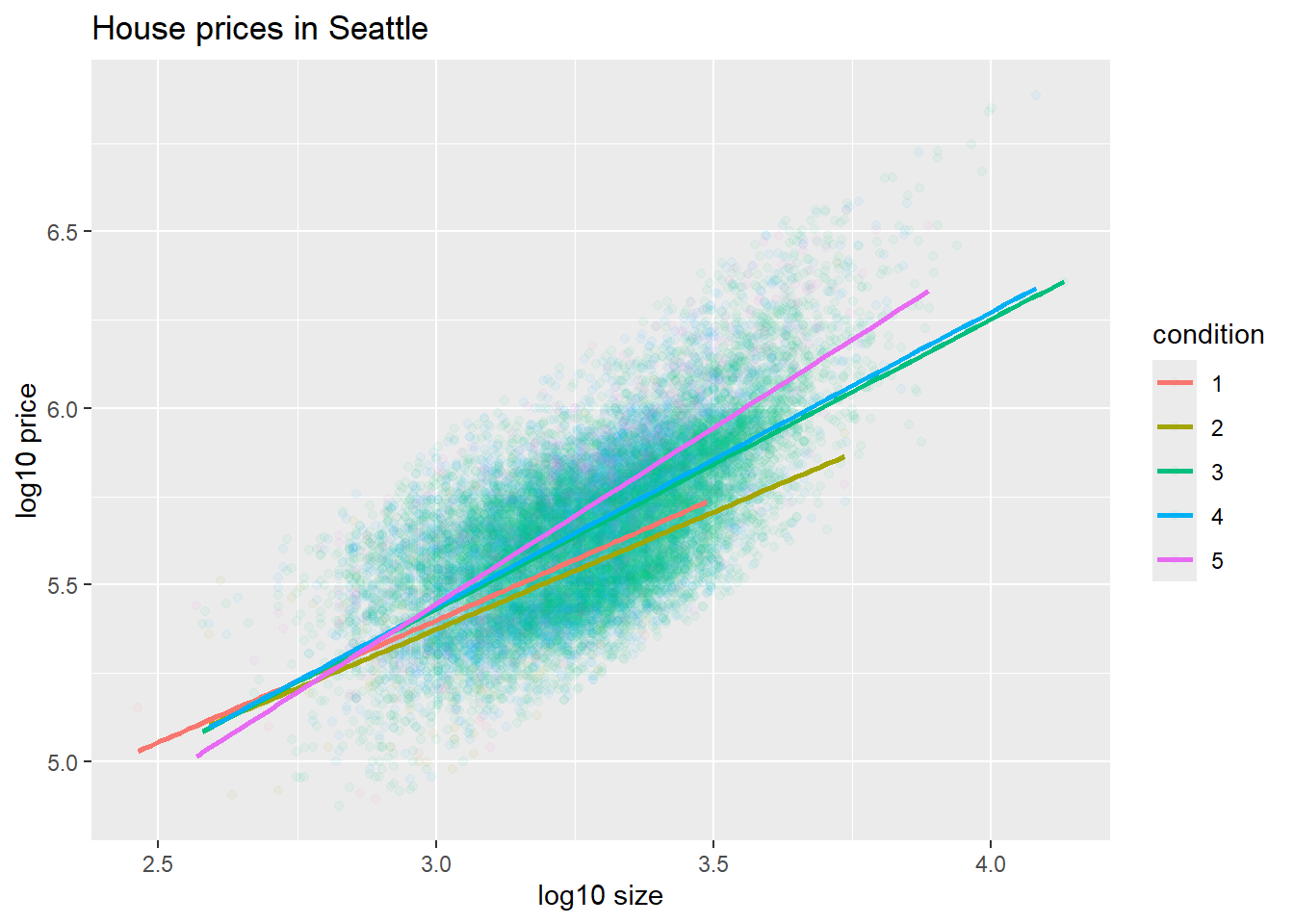

房价和房屋面积之间存在正相关关系，这意味着房屋面积越大，价格往往越高。
对于大多数房屋面积而言，状况为5的房屋似乎是最贵的。

3.1.2 回归模型建立

price_model <- lm(
  log10_price ~ log10_size * condition,
  data = house_prices_log
)
get_regression_table(price_model)

# A tibble: 10 × 7
   term                  estimate std_error statistic p_value lower_ci upper_ci
   <chr>                    <dbl>     <dbl>     <dbl>   <dbl>    <dbl>    <dbl>
 1 intercept                3.33      0.451     7.38    0        2.45     4.22 
 2 log10_size               0.69      0.148     4.65    0        0.399    0.98 
 3 condition: 2             0.047     0.498     0.094   0.925   -0.93     1.02 
 4 condition: 3            -0.367     0.452    -0.812   0.417   -1.25     0.519
 5 condition: 4            -0.398     0.453    -0.879   0.38    -1.29     0.49 
 6 condition: 5            -0.883     0.457    -1.93    0.053   -1.78     0.013
 7 log10_size:condition2   -0.024     0.163    -0.148   0.882   -0.344    0.295
 8 log10_size:condition3    0.133     0.148     0.893   0.372   -0.158    0.424
 9 log10_size:condition4    0.146     0.149     0.979   0.328   -0.146    0.437
10 log10_size:condition5    0.31      0.15      2.07    0.039    0.016    0.604

根据回归结果，我们可以建立不同条件下的回归方程，并用这些方程来预测房价。要注意的是，这些方程是基于对数变换后的变量建立的，在完成预测后还需要再进行变换才能是预测的最终值。

condition = 1: \(\hat{log10(price)} = 3.33 + 0.69 \times log10(size)\)
condition = 2: \(\hat{log10(price)} = (3.33+0.407) + (0.69-0.024)\times log10(size)\)
condition = 3: \(\hat{log10(price)} = (3.33-0.367) + (0.69+1.333)\times log10(size)\)
condition = 4: \(\hat{log10(price)} = (3.33-0.398) + (0.69+0.146)\times log10(size)\)
condition = 5: \(\hat{log10(price)} = (3.33-0.024) + (0.69+0.31) \times log10(size)\)