library(tidymodels) # for the parsnip package, along with the rest of tidymodels
library(readr) # for importing data
library(broom.mixed) # for converting bayesian models to tidy tibbles
library(dotwhisker) # for visualizing regression results4 整洁建模的一般步骤
常见的有监督学习问题为回归问题和判别问题,每一种问题都可以用许多种不同模型解决,而每一个模型都可能包含需要调优的超参数集合,对数据可能有不同的预处理、转码、函数变换、降维等变换。这些模型由许多个R扩展包实现,而且接口、选项各自不同。
tidymodels包提供了针对统计建模用户简便易用的建模功能和使用规范。R有许多建模用的扩展包,不同的扩展包在解决类似的回归、判别问题时,可能用了相近但不相同,或者完全不同的界面接口。tidymodels试图统一这些接口,使得用户可以用相同的方法调用不同的计算包。tidyr包的broom函数、nest、unnest函数提供了数据框分组建模的方便功能。
数据预处理。我们需要对数据有直观的了解,了解数据中包含哪些变量、变量的类型、变量之间的关系、变量的分布情况等。同时,我们需要对数据进行预处理,包括数据清洗、数据转换、数据降维等。
模型的建立。
- 描述性模型,如描述统计量,直方图,散点图,散点图局部曲线拟合。
- 推断性模型,如置信区间、假设检验、贝叶斯决策分析等。推断性模型的结论一般是带有概率判断的。
- 预测性模型,如回归分析、判别分析等。主要关心预测的精度。有些模型基于数学方程,如微分方程、回归模型,有些模型所需的模型假设很少,如最近邻回归。
- 模型的评估。
- 建模时,一般不仅仅考虑一个模型,而是比较多个不同模型的优劣。
- 对于同一个模型,也需要对模型的一些参数进行调整,以达到最优的效果。如lasso回归中的光滑性系数的选择,boosting(提升法)中学习速度和停止时间的选择。
- 模型的比较和参数调优经常使用交叉验证法,即将数据分成训练集和测试集,用测试集来评估模型的性能。
- 模型的表现。
- 模型的表现可以用不同的指标来衡量,如均方误差、绝对误差、R-squared、AUC、F1-score等。
- 在研究模型表现时,有可能会发现一些数据中的不足,这时有可能需要对数据进行一些新的变换,或进一步地去收集更多的数据。
- 在比较模型并筛选出少数较优模型后,应对模型的性能进行更进一步的分析,如变量之间的相关性、变量之间的交互作用、变量的重要性等。如果是预测模型,则通常需要使用建模时未使用过的数据来评估模型的预测能力。
4.1 训练集和测试集的划分
- 训练集:所有的EDA、数据预处理、模型建立、参数调整等步骤都在训练集上进行。
- 测试集:仅在模型训练完成后,使用测试集来评估模型的性能。
训练集和测试集的划分,常用如下3中方式:
从n个样本中随机抽取指定比例的样本作为训练集,剩下样本作为测试集。使用
rsample包的initial_split()函数实现。对于因变量是分类变量且类别比例相差比较悬殊的情形或者因变量未连续变量但分布重尾的情形,可以按因变量类别进行分层抽样,组成训练集,剩下样本作为测试集。在
initial_split()函数中设置strata参数为因变量(y)的名称。对于沿时间记录的数据,只能以前面一段时间为训练集,后面剩余的时间为测试集,不能选择中间的时间为测试集。使用
initial_time_split()函数实现。
Note
有些数据,如纵向数据(longitudinal data),每个受试者(观测单元)有多次观测, 这些观测不独立,需要以受试者为单位进行随机抽取,而不是以观测为单位进行抽取。
4.2 机器学习术语
预测(
prediction):预测是指根据已知的输入变量,对输出变量进行估计。预测变量(
predictor)和结果变量(outcome-variables):
- 预测变量:用于预测观测结果的变量,是已知的。
- 结果变量:如果结果是基于预测变量得到的,会在其上加一个帽子符号\(\hat{a}\);如果结果是直接观测得到的,则没有帽子符号。
模型(
model):模型是对输入-输出关系的一种描述,是对输入变量和输出变量之间关系的一种假设。拟合模型(
fitted-model)和非拟合模型(unfitted-model):
- 拟合模型:模型在训练集上进行训练得到的模型,是对真实模型的一种近似。
- 非拟合模型:模型参数未经过训练,即模型的参数未知。非拟合模型不能用于预测。
参数(
parameter):机器学习算法根据预先设定的目标,通过优化算法寻找最优参数,这些参数是模型的输入。训练集(
training-set)和测试集(test-set):
- 训练集:用于训练模型的样本集合,通过对模型的训练,努力使预测误差最小化。
- 测试集:用于评估模型性能的样本集合,模型在测试集上进行评估,评估模型的泛化能力。
5 使用tidymodels进行机器学习的简单实例
5.1 定义模型
这部分相关内容在 Chapter 5 中有详细介绍。
5.1.1 载入并初步了解数据
# load data
urchins <-
  read_csv("D:/Document/0.Study R/6.Tidymodels-with-R/data/urchins.csv") |>
  rename(food_regime = TREAT, initial_volume = IV, width = SUTW) |>
  mutate(
    food_regime = factor(food_regime, levels = c("Initial", "Low", "High"))
  )

# plot data
ggplot(
  urchins,
  aes(x = initial_volume, y = width, group = food_regime, color = food_regime)
) +
  geom_point() +
  geom_smooth(method = "lm", se = FALSE) +
  scale_color_viridis_d(option = "plasma") +
  theme_bw() +
  theme(legend.position = "top")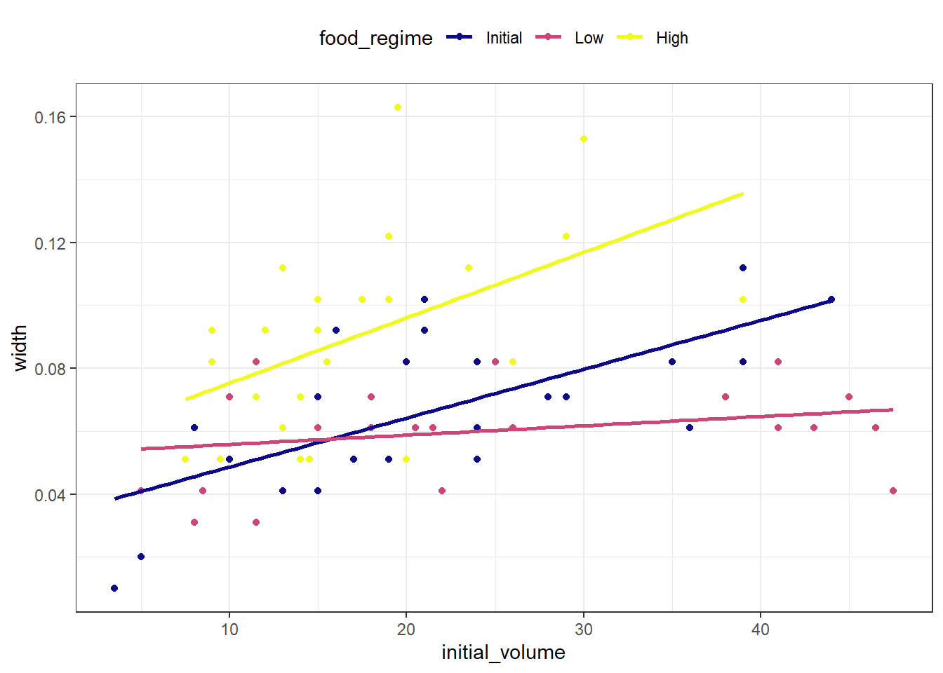
在实验开始时体积较大的海胆在最后往往有更宽的缝合,但是线条的斜率看起来不同,所以这种效果可能取决于摄食条件。
5.1.2 建立模型
线性回归(最小二乘法)是建立最初模型的好选择。 这里我们使用parsnip包中的linear_reg()函数来定义线性回归模型, 并使用set_engine()来指定模型的引擎,即模型的算法。
# define model
lm_mod <-
  linear_reg() |>
  set_engine("lm")
lm_mod
Linear Regression Model Specification (regression)
Computational engine: lm # fit model
lm_fit <-
lm_mod |>
fit(width ~ initial_volume * food_regime, data = urchins)
lm_fitparsnip model object
Call:
stats::lm(formula = width ~ initial_volume * food_regime, data = data)
Coefficients:
(Intercept) initial_volume
0.0331216 0.0015546
food_regimeLow food_regimeHigh
0.0197824 0.0214111
initial_volume:food_regimeLow initial_volume:food_regimeHigh
-0.0012594 0.0005254 # use broom.mixed to get a tidy summary of the model
tidy(lm_fit)# A tibble: 6 × 5
term estimate std.error statistic p.value
<chr> <dbl> <dbl> <dbl> <dbl>
1 (Intercept) 0.0331 0.00962 3.44 0.00100
2 initial_volume 0.00155 0.000398 3.91 0.000222
3 food_regimeLow 0.0198 0.0130 1.52 0.133
4 food_regimeHigh 0.0214 0.0145 1.47 0.145
5 initial_volume:food_regimeLow -0.00126 0.000510 -2.47 0.0162
6 initial_volume:food_regimeHigh 0.000525 0.000702 0.748 0.457 # visualize the model coefficients with dotwhisker
dwplot(
lm_fit,
dot_args = list(size = 2, color = "black"),
whisker_args = list(color = "black"),
vline = geom_vline(xintercept = 0, color = "grey50", linetype = 2)
) +
theme_bw()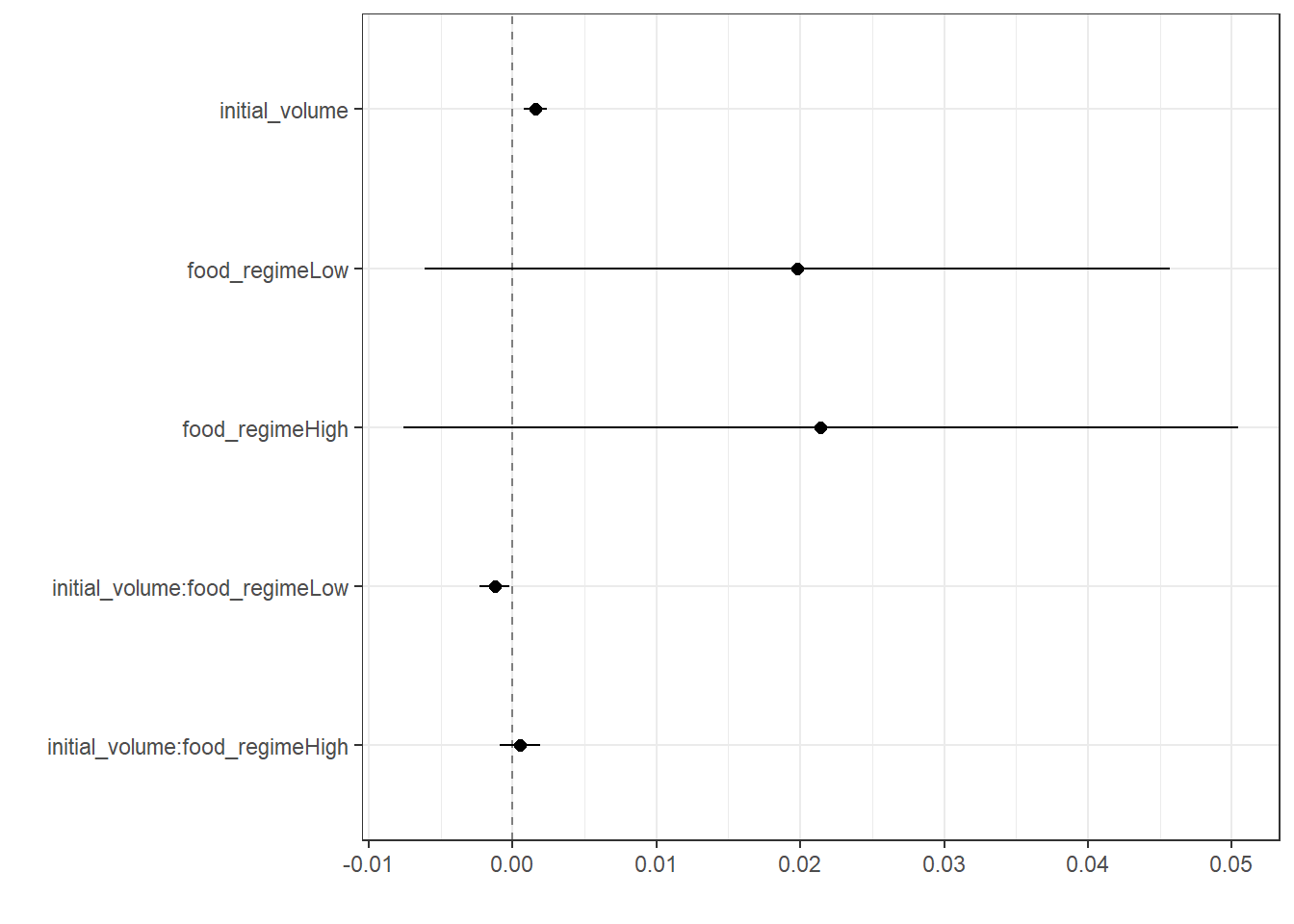
5.1.3 模型预测
生成一个新的数据集来预测不同初始体积和食物条件下的缝合宽度(假设新数据的海胆是以20ml的初始体积开始试验的)。
# define new data
new_uchins <-
  expand.grid(
    initial_volume = 20,
    food_regime = c("Initial", "Low", "High")
  )
new_uchins
initial_volume food_regime
1 20 Initial
2 20 Low
3 20 High对新数据进行预测,并将预测结果添加到新数据集中。
# 生成预测值
mean_pred <- predict(lm_fit, new_data = new_uchins)
mean_pred
# A tibble: 3 × 1
.pred
<dbl>
1 0.0642
2 0.0588
3 0.0961# 生成置信区间
conf_int_pred <- predict(lm_fit, new_data = new_uchins, type = "conf_int")
conf_int_pred# A tibble: 3 × 2
.pred_lower .pred_upper
<dbl> <dbl>
1 0.0555 0.0729
2 0.0499 0.0678
3 0.0870 0.105 # 将预测值和置信区间添加到新数据集中
pred_data <-
new_uchins |>
bind_cols(mean_pred) |>
bind_cols(conf_int_pred)
pred_data initial_volume food_regime .pred .pred_lower .pred_upper
1 20 Initial 0.06421443 0.05549934 0.07292952
2 20 Low 0.05880940 0.04986251 0.06775629
3 20 High 0.09613343 0.08696233 0.10530453# 绘制预测图形
ggplot(pred_data, aes(x = food_regime)) +
geom_point(aes(y = .pred)) +
geom_errorbar(aes(ymin = .pred_lower, ymax = .pred_upper), width = 0.2) +
labs(y = "urchin size") +
theme_bw()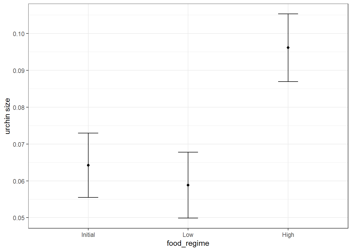
5.1.4 使用其他模型算法
我们可能会有兴趣知道如果使用贝叶斯方法估计模型,结果是否会有所不同。在这样的分析中,需要为每个模型参数声明一个先验分布,该参数代表参数的可能值(在暴露于观察到的数据之前)。
我们假设这个先验分布是钟形的,同时因为不清楚分布的具体范围,在设定先验分布时可采取保守的方法,使得先验分布的宽度尽量变宽。
# set prior distributions
prior_dist <- rstanarm::student_t(df = 1)

set.seed(123)

# define bayesian model
bayes_model <-
  linear_reg() |>
  set_engine("stan", prior_intercept = prior_dist, prior = prior_dist)
bayes_model
Linear Regression Model Specification (regression)
Engine-Specific Arguments:
prior_intercept = prior_dist
prior = prior_dist
Computational engine: stan # fit bayesian model
bayes_fit <-
bayes_model |>
fit(width ~ initial_volume * food_regime, data = urchins)
bayes_fitparsnip model object
stan_glm
family: gaussian [identity]
formula: width ~ initial_volume * food_regime
observations: 72
predictors: 6
------
Median MAD_SD
(Intercept) 0.0 0.0
initial_volume 0.0 0.0
food_regimeLow 0.0 0.0
food_regimeHigh 0.0 0.0
initial_volume:food_regimeLow 0.0 0.0
initial_volume:food_regimeHigh 0.0 0.0
Auxiliary parameter(s):
Median MAD_SD
sigma 0.0 0.0
------
* For help interpreting the printed output see ?print.stanreg
* For info on the priors used see ?prior_summary.stanreg# use broom.mixed to get a tidy summary of the model
tidy(bayes_fit, conf.int = TRUE)# A tibble: 6 × 5
term estimate std.error conf.low conf.high
<chr> <dbl> <dbl> <dbl> <dbl>
1 (Intercept) 0.0330 0.00983 0.0165 0.0488
2 initial_volume 0.00155 0.000401 0.000899 0.00225
3 food_regimeLow 0.0203 0.0133 -0.00165 0.0420
4 food_regimeHigh 0.0211 0.0147 -0.00243 0.0459
5 initial_volume:food_regimeLow -0.00128 0.000508 -0.00212 -0.000411
6 initial_volume:food_regimeHigh 0.000535 0.000712 -0.000656 0.00171 # predict using bayesian model and polt results
bayes_pred <-
new_uchins |>
bind_cols(predict(bayes_fit, new_data = new_uchins)) |>
bind_cols(predict(bayes_fit, new_data = new_uchins, type = "conf_int"))
bayes_pred initial_volume food_regime .pred .pred_lower .pred_upper
1 20 Initial 0.06417657 0.05575406 0.07274127
2 20 Low 0.05884211 0.04972501 0.06772253
3 20 High 0.09611819 0.08704594 0.10505292ggplot(bayes_pred, aes(x = food_regime)) +
geom_point(aes(y = .pred)) +
geom_errorbar(aes(ymin = .pred_lower, ymax = .pred_upper), width = 0.2) +
labs(y = "urchin size") +
theme_bw()
5.2 预处理
这部分相关内容在 Chapter 7,Chapter 9,Chapter 6 中有详细介绍。
library(tidymodels) # for the recipes package, along with the rest of tidymodels

# Helper packages
library(nycflights13) # for flight data
library(skimr) # for variable summaries

set.seed(123)

flight_data <-
  flights %>%
  mutate(
    # Convert the arrival delay to a factor
    arr_delay = ifelse(arr_delay >= 30, "late", "on_time"),
    arr_delay = factor(arr_delay),
    # We will use the date (not date-time) in the recipe below
    date = lubridate::as_date(time_hour)
  ) %>%
  # Include the weather data
  inner_join(weather, by = c("origin", "time_hour")) %>%
  # Only retain the specific columns we will use
  select(
    dep_time,
    flight,
    origin,
    dest,
    air_time,
    distance,
    carrier,
    date,
    arr_delay,
    time_hour
  ) %>%
  # Exclude missing data
  na.omit() %>%
  # For creating models, it is better to have qualitative columns
  # encoded as factors (instead of character strings)
  mutate_if(is.character, as.factor)
flight_data
# A tibble: 325,819 × 10
dep_time flight origin dest air_time distance carrier date arr_delay
<int> <int> <fct> <fct> <dbl> <dbl> <fct> <date> <fct>
1 517 1545 EWR IAH 227 1400 UA 2013-01-01 on_time
2 533 1714 LGA IAH 227 1416 UA 2013-01-01 on_time
3 542 1141 JFK MIA 160 1089 AA 2013-01-01 late
4 544 725 JFK BQN 183 1576 B6 2013-01-01 on_time
5 554 461 LGA ATL 116 762 DL 2013-01-01 on_time
6 554 1696 EWR ORD 150 719 UA 2013-01-01 on_time
7 555 507 EWR FLL 158 1065 B6 2013-01-01 on_time
8 557 5708 LGA IAD 53 229 EV 2013-01-01 on_time
9 557 79 JFK MCO 140 944 B6 2013-01-01 on_time
10 558 301 LGA ORD 138 733 AA 2013-01-01 on_time
# ℹ 325,809 more rows
# ℹ 1 more variable: time_hour <dttm># 计算晚点超过30min的航班数量
flight_data |>
count(arr_delay) |>
mutate(prop = n / sum(n))# A tibble: 2 × 3
arr_delay n prop
<fct> <int> <dbl>
1 late 52540 0.161
2 on_time 273279 0.839在构建预处理配方之前,我们需要关注一下对预处理和建模有影响的变量:
-
arr_delay变量,是一个分类变量,表示航班是否晚点超过30分钟,这是我们的结果变量。 -
flight和time_hour是我们不希望在模型中作为预测变量使用的两个变量,但我们希望保留它们作为识别变量,可用于对预测不佳的数据点进行故障排除。 -
dest变量包含104个dest和16个不同的carriers。这两个变量是因子类型,所以在模型中使用时需要转换为虚拟变量形式。但是,两个变量变量的水平数均比较多,直接转换为虚拟变量会导致模型过于复杂,且部分因子水平出现的次数很少。所以我们需要对它们进行一些处理。
flight_data |>
skimr::skim(dest, carrier)| Name | flight_data |
| Number of rows | 325819 |
| Number of columns | 10 |
| _______________________ | |
| Column type frequency: | |
| factor | 2 |
| ________________________ | |
| Group variables | None |
Variable type: factor
| skim_variable | n_missing | complete_rate | ordered | n_unique | top_counts |
|---|---|---|---|---|---|
| dest | 0 | 1 | FALSE | 104 | ATL: 16771, ORD: 16507, LAX: 15942, BOS: 14948 |
| carrier | 0 | 1 | FALSE | 16 | UA: 57489, B6: 53715, EV: 50868, DL: 47465 |
5.2.1 数据划分
将这个单个数据集分成两个: 训练集和测试集。将原始数据集中的大部分行(随机选择的子集)保留在训练集中。训练数据将用于拟合模型, 测试集将用于测量模型性能。 Chapter 9。
set.seed(222)

data_split <- initial_split(flight_data, prop = 3 / 4)

train_data <- training(data_split)
test_data <- testing(data_split)
5.2.2 定义预处理配方并进行特征工程
recipe()函数定义了预处理配方的基本结构。 - 第一个参数是一个公式,指定了结果变量和预测变量。 - 第二个参数是数据集。通常为训练集。 - 使用update_role()函数指定变量的角色,例如将flight和time_hour变量的角色更新为“ID”,表示它们是识别变量,不用于建模。
当模型拟合完成后,我们想关注一些预测不佳的值并尝试解决预测结果不佳的问题时,这些ID列就会很有用。
flights_rec <-
  recipe(arr_delay ~ ., data = train_data) |>
  update_role(flight, time_hour, new_role = "ID") |>
  # 创建新因子列,包含对应的星期数和月份
  step_date(date, features = c("dow", "month")) |>
  # 创建一个变量,标识当前日期是否为节假日
  step_holiday(
    date,
    holidays = timeDate::listHolidays("US"),
    keep_original_cols = FALSE
  ) |>
  # 将所有因子变量转换为虚拟变量
  step_dummy(all_nominal_predictors()) |>
  # 删除所有预测变量中只出现一次的水平
  step_zv(all_predictors())
flights_rec
5.2.3 Fit a model with a recipe
在创建recipe后,将其拟合到模型中,告诉模型应该如何处理数据。
# define model
lr_mod <-
  logistic_reg() |>
  set_engine("glm")

# define workflow to combine models and recipes
flight_wflow <-
  workflow() |>
  add_model(lr_mod) |>
  add_recipe(flights_rec)
flight_wflow
══ Workflow ════════════════════════════════════════════════════════════════════
Preprocessor: Recipe
Model: logistic_reg()
── Preprocessor ────────────────────────────────────────────────────────────────
4 Recipe Steps
• step_date()
• step_holiday()
• step_dummy()
• step_zv()
── Model ───────────────────────────────────────────────────────────────────────
Logistic Regression Model Specification (classification)
Computational engine: glm # fit the workflow to the training data
flight_fit <-
flight_wflow |>
fit(data = train_data)
# extract the prepped recipe from the fitted workflow
flight_fit |>
extract_recipe() |>
tidy()# A tibble: 4 × 6
number operation type trained skip id
<int> <chr> <chr> <lgl> <lgl> <chr>
1 1 step date TRUE FALSE date_7pdqb
2 2 step holiday TRUE FALSE holiday_kl2Li
3 3 step dummy TRUE FALSE dummy_jB5fX
4 4 step zv TRUE FALSE zv_VpqIE # extract the fitted model from the fitted workflow
flight_fit |>
extract_fit_parsnip() |>
tidy()# A tibble: 157 × 5
term estimate std.error statistic p.value
<chr> <dbl> <dbl> <dbl> <dbl>
1 (Intercept) 7.28 2.73 2.67 7.64e- 3
2 dep_time -0.00166 0.0000141 -118. 0
3 air_time -0.0440 0.000563 -78.2 0
4 distance 0.00507 0.00150 3.38 7.32e- 4
5 date_USChristmasDay 1.33 0.177 7.49 6.93e-14
6 date_USColumbusDay 0.724 0.170 4.25 2.13e- 5
7 date_USCPulaskisBirthday 0.807 0.139 5.80 6.57e- 9
8 date_USDecorationMemorialDay 0.585 0.117 4.98 6.32e- 7
9 date_USElectionDay 0.948 0.190 4.98 6.25e- 7
10 date_USGoodFriday 1.25 0.167 7.45 9.40e-14
# ℹ 147 more rows5.2.4 对训练后的workflow进行预测
# use predict()
predict(flight_fit, new_data = test_data)
# A tibble: 81,455 × 1
.pred_class
<fct>
1 on_time
2 on_time
3 on_time
4 on_time
5 on_time
6 on_time
7 on_time
8 on_time
9 on_time
10 on_time
# ℹ 81,445 more rows# use augment() to add predictions to the test data-recommended
flight_aug <-
augment(flight_fit, new_data = test_data)
flight_aug |>
select(arr_delay, .pred_class, .pred_on_time:.pred_late)# A tibble: 81,455 × 4
arr_delay .pred_class .pred_on_time .pred_late
<fct> <fct> <dbl> <dbl>
1 on_time on_time 0.945 0.0547
2 on_time on_time 0.949 0.0515
3 on_time on_time 0.964 0.0361
4 on_time on_time 0.961 0.0386
5 on_time on_time 0.962 0.0384
6 on_time on_time 0.975 0.0249
7 on_time on_time 0.963 0.0366
8 on_time on_time 0.981 0.0191
9 on_time on_time 0.935 0.0646
10 on_time on_time 0.931 0.0687
# ℹ 81,445 more rows5.2.5 评估模型
flight_aug |>
  # 计算ROC曲线
  roc_curve(truth = arr_delay, .pred_late) |>
  autoplot()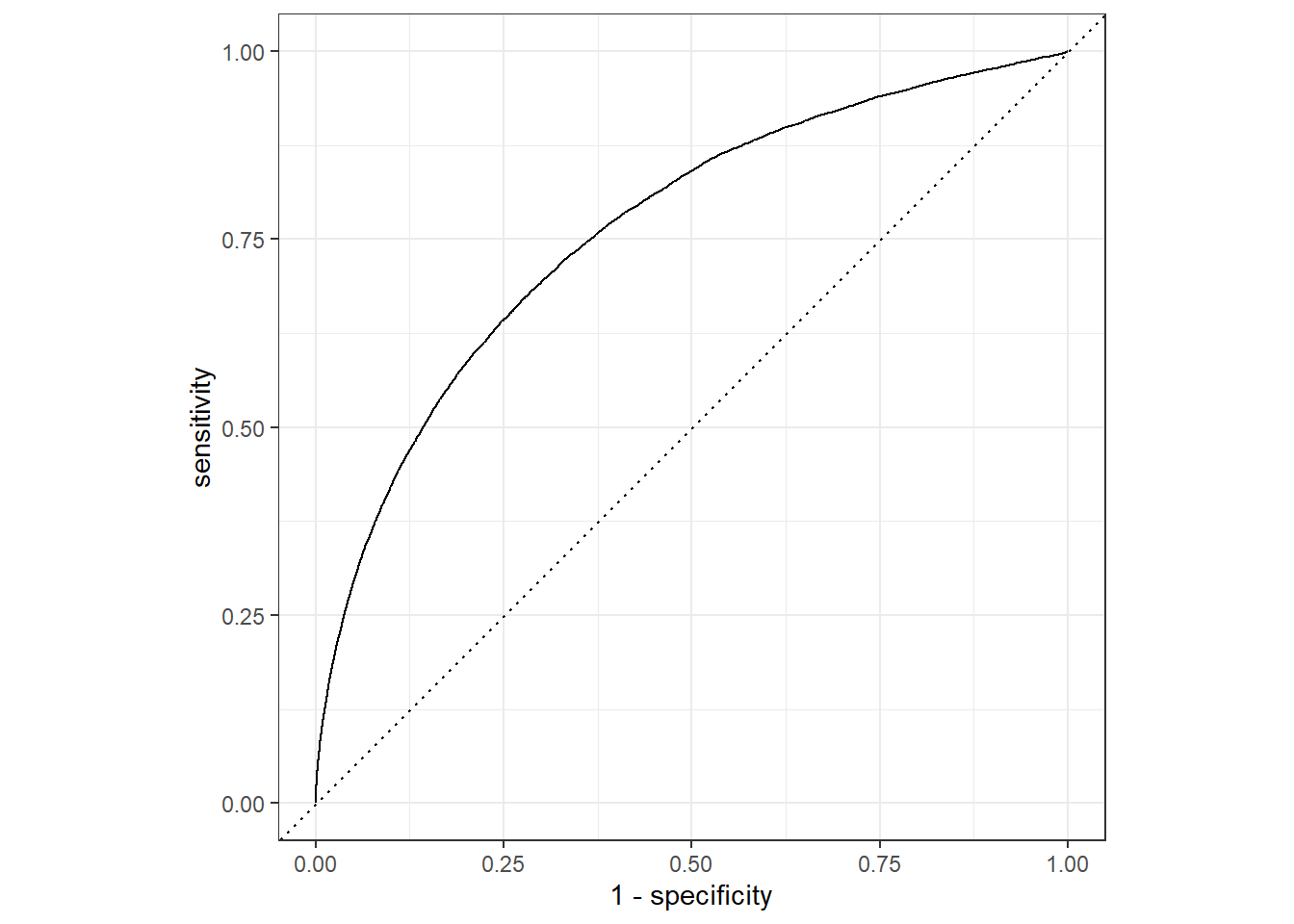
未来我们将持续深入的了解tidymodels包的各个组件, 包括parsnip(Chapter 5) 、recipes(Chapter 7)、 workflows(Chapter 6, Chapter 14)、 tune(Chapter 11)、 rsample(Chapter 9)、 yardstick(Chapter 8) 等, 以及如何使用tidymodels实现各种机器学习算法。