1 抽样、估计、置信区间

library(tidyverse)
library(infer)
library(moderndive)

1.1 抽样相关的基本概念

总体 (population): 研究对象的全体。
样本 (sample): 从总体中抽取的一部分。
参数 (parameter): 描述总体的数值特征。
统计量 (statistic): 描述样本的数值特征。
抽样分布 (sampling distribution): 统计量在所有可能的样本中的分布。
中心极限定理 (Central Limit Theorem): 当样本量足够大时，样本均值的抽样分布趋近于正态分布。可参看我的博文。

Note

标准差(sd)：方差¹的平方根。总体标准差的分母是n，样本标准差的分母是n-1。 在R中，直接使用sd()函数计算样本标准差。
标准误差(标准误)(se)：方差的均值的算术平方根。也就是标准差除以样本量的平方根。标准误反映了统计量的变异程度。标准误越小，统计量越稳定。

1.2 置信区间 (Confidence Interval)

置信区间是用来估计总体参数的范围。它由两个数值组成，表示在一定置信水平下，总体参数落在该范围内的概率。

置信区间的手动计算步骤如下：

计算样本均值 \(\bar{x}\) 和样本标准误差 \(SE\)。
确定需要的置信水平(例如常用的95%的置信水平)，确定对应的z分数值(表示相差多少个标准差)。
计算置信区间，\(CI_{low} = \bar{x} - z \times SE\), \(CI_{high} = \bar{x} + z \times SE\)。
解释置信区间。

\(SE = 样本标准差 \sqrt{n}\)

1.3 利用infer包进行bootstrap估计 (Estimation)

在实际中，我们通常无法获取总体的全部数据，因此需要通过样本数据来估计总体参数。这个过程称为估计 (Estimation)，也是统计和数据科学的核心之一。

Bootstrap 是一种基于重抽样的统计方法，通过对原始样本进行有放回的重复抽样，生成大量 Bootstrap 样本，进而用于估计总体参数、标准误差等，以实现构建置信区间、执行假设检验等统计推断任务。

本节简单介绍使用infer包进行Bootstrap估计的基本工作流程。

infer的主要函数可参看inferd的官方文档。

bootstrap_means <- almonds_sample_100 |>
  specify(response = weight) |> # 指定响应变量
  generate(reps = 1000, type = "bootstrap") |> # 生成1000个bootstrap样本
  calculate(stat = "mean") # 计算样本均值
bootstrap_means

Response: weight (numeric)
# A tibble: 1,000 × 2
   replicate  stat
       <int> <dbl>
 1         1  3.72
 2         2  3.70
 3         3  3.70
 4         4  3.67
 5         5  3.64
 6         6  3.62
 7         7  3.67
 8         8  3.69
 9         9  3.68
10        10  3.68
# ℹ 990 more rows

visualise(bootstrap_means) # 快速可视化结果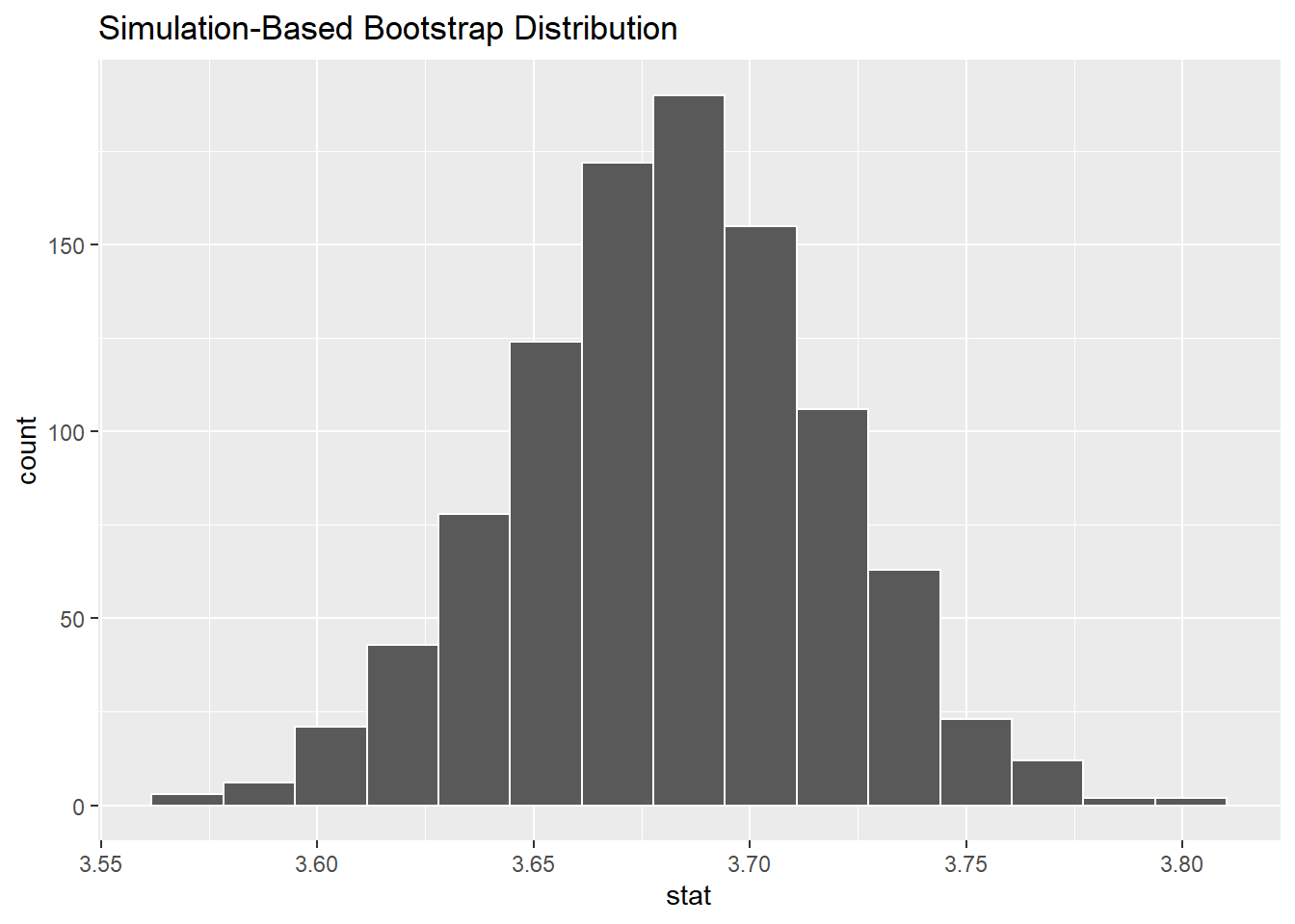

1.3.1 利用infer包进行bootstrap样本的置信区间计算

我们只需在上面的代码基础上，使用get_confidence_interval()函数即可。

get_confidence_interval()函数中可以通过type参数方便的切换置信区间的计算方法

# 使用percentile方法计算95%的置信区间
percentile_ci <- bootstrap_means |>
  get_ci(level = 0.95, type = "percentile")
percentile_ci

# A tibble: 1 × 2
  lower_ci upper_ci
     <dbl>    <dbl>
1     3.61     3.75

# 可视化结果
visualise(bootstrap_means) +
  shade_ci(endpoints = percentile_ci, color = "hotpink", fill = "khaki")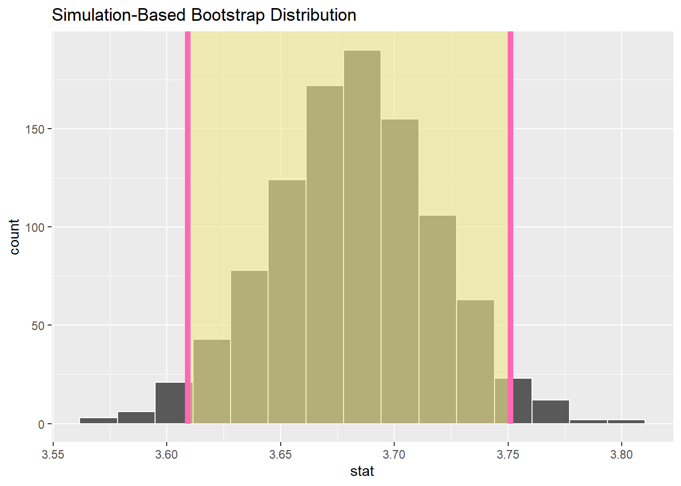

# 使用se方法计算95%的置信区间
# se方法基于正态分布假设，需要计算原始样本的均值
x_bar <- almonds_sample_100 |>
  specify(response = weight) |>
  calculate(stat = "mean")
x_bar

Response: weight (numeric)
# A tibble: 1 × 1
   stat
  <dbl>
1  3.68

se_ci <- bootstrap_means |>
  get_ci(level = 0.95, type = "se", point_estimate = x_bar)
se_ci

# A tibble: 1 × 2
  lower_ci upper_ci
     <dbl>    <dbl>
1     3.61     3.75

# 可视化结果
visualise(bootstrap_means) +
  shade_ci(endpoints = se_ci, color = "blue", fill = "lightblue")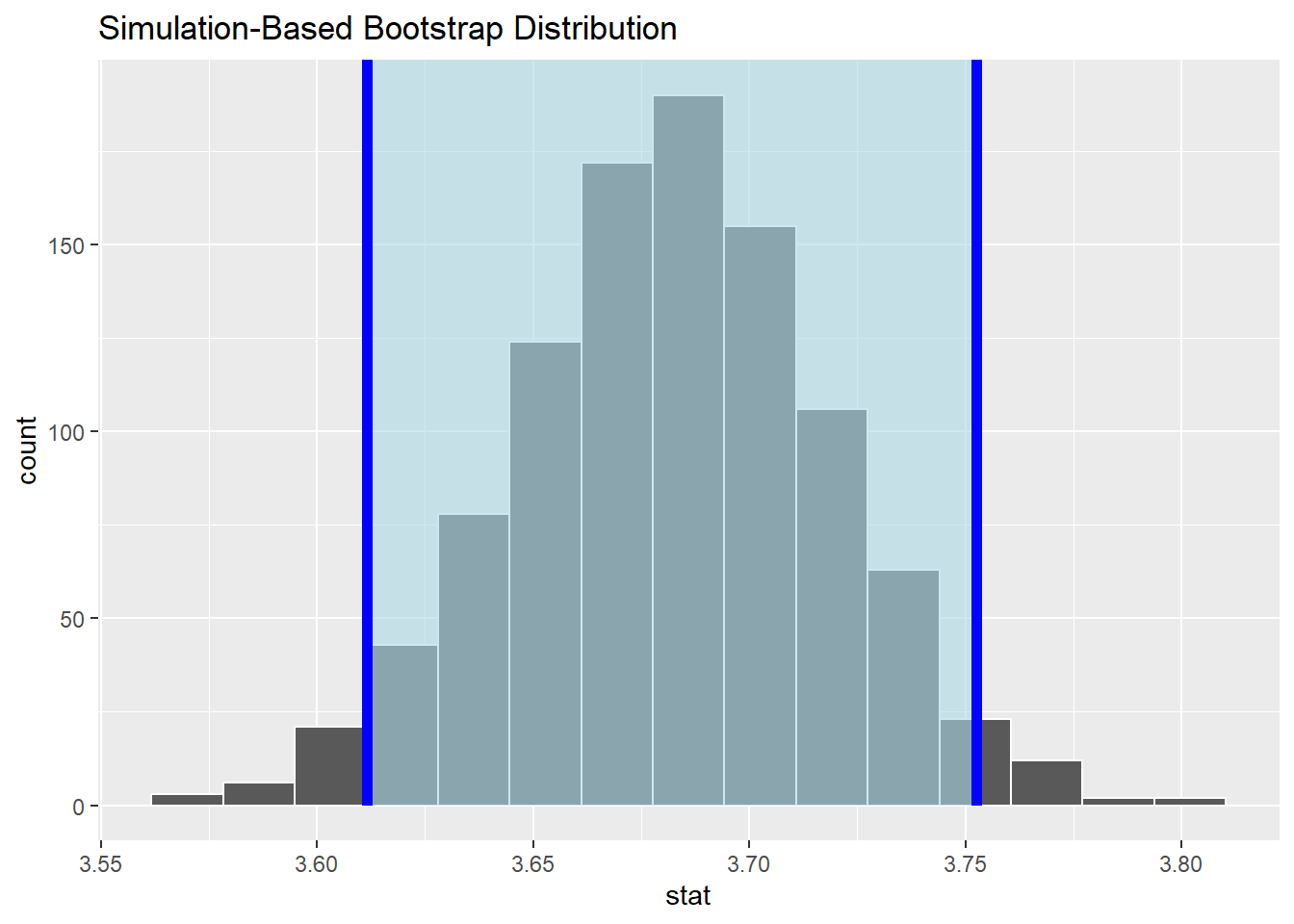

1.4 案例-打哈欠会传染吗？

mythbusters_yawn

# A tibble: 50 × 3
    subj group   yawn 
   <int> <chr>   <chr>
 1     1 seed    yes  
 2     2 control yes  
 3     3 seed    no   
 4     4 seed    yes  
 5     5 seed    no   
 6     6 control no   
 7     7 seed    yes  
 8     8 control no   
 9     9 control no   
10    10 seed    no   
# ℹ 40 more rows

# Constructing the CI
yawn_bootstrap <- mythbusters_yawn |>
  # 指定变量和成功类别
  specify(formula = yawn ~ group, success = "yes") |>
  # 生成重复样本
  generate(reps = 1000, type = "bootstrap") |>
  calculate(stat = "diff in props", order = c("seed", "control"))
yawn_bootstrap

Response: yawn (factor)
Explanatory: group (factor)
# A tibble: 1,000 × 2
   replicate     stat
       <int>    <dbl>
 1         1 -0.0457 
 2         2  0.0903 
 3         3  0.210  
 4         4  0.124  
 5         5  0.139  
 6         6  0.110  
 7         7  0.105  
 8         8 -0.0286 
 9         9  0.129  
10        10 -0.00794
# ℹ 990 more rows

# 计算置信区间
yawn_bootstrap_ci <- yawn_bootstrap |>
  get_ci(type = "percentile", level = 0.95)
yawn_bootstrap_ci

# A tibble: 1 × 2
  lower_ci upper_ci
     <dbl>    <dbl>
1   -0.208    0.312

# 可视化结果

visualise(yawn_bootstrap) +
  shade_ci(endpoints = yawn_bootstrap_ci, color = "purple", fill = "plum") +
  geom_vline(xintercept = 0, linetype = "dashed", color = "yellow")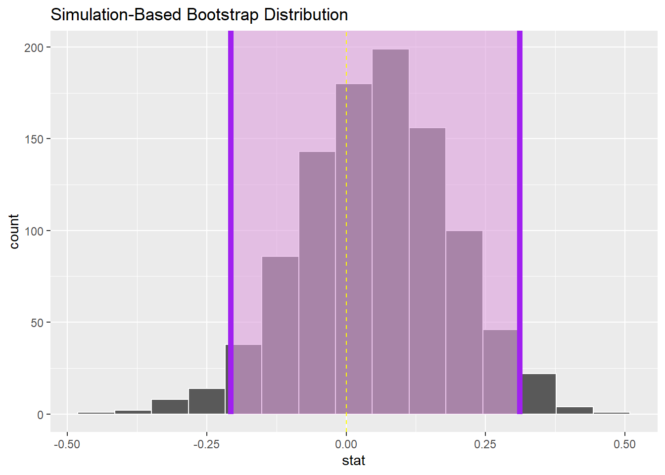

置信区间包括0值，说明我们无法确定两组测试人员之间的打哈欠的比例是否有区别，侧面说明打哈欠传染的效果不显著。
假设 95% 置信区间完全高于零，表明 pseed−pcontrol>0 ，或者换句话说 pseed>pcontrol ，则有证据有证据表明那些打哈欠的人确实更频繁地打哈欠。

1.5 小结

我们已经了解了抽样、估计和置信区间的基本概念，并学习了如何使用infer包进行Bootstrap估计和置信区间的计算。这些工具和方法在统计分析和数据科学中非常重要，能够帮助我们从样本数据中推断总体特征。那么，接下来我们将学习如何进行假设检验，以进一步验证我们的统计推断。

方差(SS)是数据与其均值之差的平方和的平均值。方差越大，数据分布越分散；方差越小，数据越集中。↩︎